Hierarchical Stock Recruitment Analysis
Stan program for Hierarchical Stock-recruitment analysis (with covariates Latitude) Chapter 9 - section 9.3
hierarchical-stock-recruitment.Rmd
library(hbm4ecology)
#> Please visit the site https://Chabert-Liddell.github.io/hbm4ecology/articles/
#>                           for R case study.
library(rstan)
#> Loading required package: StanHeaders
#> Loading required package: ggplot2
#> rstan (Version 2.21.5, GitRev: 2e1f913d3ca3)
#> For execution on a local, multicore CPU with excess RAM we recommend calling
#> options(mc.cores = parallel::detectCores()).
#> To avoid recompilation of unchanged Stan programs, we recommend calling
#> rstan_options(auto_write = TRUE)
library(posterior)
#> This is posterior version 1.2.1
#>
#> Attaching package: 'posterior'
#> The following objects are masked from 'package:rstan':
#>
#>     ess_bulk, ess_tail
#> The following objects are masked from 'package:stats':
#>
#>     mad, sd, var
library(tidyverse)
#> ── Attaching packages ─────────────────────────────────────── tidyverse 1.3.1 ──
#> ✔ tibble  3.1.7     ✔ dplyr   1.0.9
#> ✔ tidyr   1.2.0     ✔ stringr 1.4.0
#> ✔ readr   2.1.2     ✔ forcats 0.5.1
#> ✔ purrr   0.3.4
#> ── Conflicts ────────────────────────────────────────── tidyverse_conflicts() ──
#> ✖ tidyr::extract() masks rstan::extract()
#> ✖ dplyr::filter()  masks stats::filter()
#> ✖ dplyr::lag()     masks stats::lag()
#plot_theme <- theme_set(theme_classic(base_size = 15L))
plot_theme <-  theme_classic(base_size = 15L) +
  theme(axis.text.x =  element_text(angle = 90),
        strip.background = element_rect(fill = "#4da598"),
        strip.text = element_text(size = 15))
This article develops a hierarchical extension of the Ricker Stock Recruitment model. The data and models are based on a published paper by Pr{'{e}}vost et al. Prévost et al. (2003); but see also Prévost, Chaput, and (Ed.) (2001).
We show that the hierarchical assemblage of several salmon populations which we model as exchangeable units appears as the working solution to transfer information and borrow strength from data-rich to data-poor situations. The data structure is sophisticated with Normal latent vectors, and the probabilistic structures have to be designed conditionally on some available covariates, namely the latitude and the riverine wetted area accessible to salmon.
Data
data("SRSalmon")The analysis of stock and recruitment (SR) relationships is the most widely used approach for deriving Biological Reference Points in fisheries sciences. It is particularly well suited for anadromous salmonid species for which the recruitment of juveniles in freshwater is more easily measured than the recruitment of marine species. SR relationships are critical for setting reference points for the management of salmon populations, such as the spawning target \(S^{\ast}\), a biological reference point for the number of spawners which are necessary to guarantee an optimal sustainable exploitation, or the maximum sustainable exploitation rate \(h^{\ast}\).
tibble(
  River = SRSalmon$name_riv,
  Country = SRSalmon$country_riv,
  Latitude = SRSalmon$lat,
  `Area accessible to salmon` = SRSalmon$area
) %>% knitr::kable()| River | Country | Latitude | Area accessible to salmon |
|---|---|---|---|
| Nivelle | France | 43.50000 | 320995 |
| Oir | France | 48.50000 | 48000 |
| Frome | England | 50.50000 | 876420 |
| Dee | England | 53.00000 | 6170000 |
| Burrishoole | Ireland | 53.98515 | 155000 |
| Lune | England | 54.50000 | 4230000 |
| Bush | N. Ireland | 55.00000 | 845500 |
| Mourne | N. Ireland | 55.00000 | 10360560 |
| Faughan | N. Ireland | 55.00000 | 882380 |
| Girnock Burn | Scotland | 57.00000 | 58764 |
| North Esk | Scotland | 57.00000 | 2100000 |
| Laerdalselva | Norway | 61.00000 | 704000 |
| Ellidaar | Iceland | 64.00000 | 199711 |
tib <- tibble(Obs = seq(SRSalmon$n),
              River = SRSalmon$riv,
              Stock = SRSalmon$S,
              Recruitment = SRSalmon$R)
knitr::kable(bind_rows(head(tib), tail(tib)))| Obs | River | Stock | Recruitment |
|---|---|---|---|
| 1 | 1 | 0.957 | 2.647 |
| 2 | 1 | 0.501 | 0.444 |
| 3 | 1 | 2.286 | 1.801 |
| 4 | 1 | 1.481 | 0.573 |
| 5 | 1 | 1.596 | 0.356 |
| 6 | 1 | 2.679 | 0.390 |
| 134 | 13 | 37.955 | 111.579 |
| 135 | 13 | 42.157 | 139.799 |
| 136 | 13 | 32.309 | 124.208 |
| 137 | 13 | 34.869 | 85.049 |
| 138 | 13 | 24.022 | 73.261 |
| 139 | 13 | 31.268 | 71.534 |
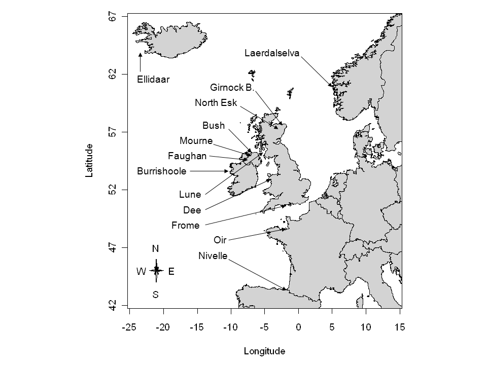
Location of the 13 index rivers with available stock-recruitment datasets for A. salmon (from Prévost et al. (2003)).
There are several hundreds of salmon stocks in the northeast Atlantic
area, each having its own characteristics with regard to the size and
productivity of the salmon populations. But resources to collect SR data
are limited and suitable SR series (both in terms of length and
reliability of observations) such as the ones of SRSalmon
are only available for a handful of monitored rivers spread throughout
the European area of distribution of the species. These so-called
index rivers are a representative sample from the salmon rivers
located in western Europe and under the influence of the Gulf Stream.
This sample covers a broad area including Spain, France, UK, Ireland,
Norway, the western coast of Sweden and the southwestern coast of
Iceland. The collection and pre-processing procedures used to obtain the
data ready for SR analysis presented in Table
are described in detail in Crozier et al. (2003) or Prévost et al. (2003). Here, hierarchical modeling will
be used to address two questions:
- How is the SR information transferred from the monitored data-rich rivers to set Biological Reference Points for other sparse-data salmon rivers, while accounting for the major sources of uncertainty?
- How can the joint analysis of the SR relationship for the 13 index rivers be used to forecast biological reference points for a new river without any SR data but for which relevant covariates are available?
Model without covariates
Ricker model with lognormal errors and management related parametrization
- \(\log(R_{k,t}) = h_{k}^{*} + \log(\frac{S_{k,t}}{1-h^{*}{t}}) - \frac{h^{*}_{k}}{S^{*}_{k}}S_{k,t} + \epsilon_{k,t}\)
- \(\epsilon_{k,t} \overset{iid}{\sim} Normal(0, \sigma_k^2)\)
Defining priors for the model
- \(h_k^* \sim Beta(1,1)\)
- \(\tau = \sigma^{-2} \sim Gamma(p = 10^{-3},q = 10^{-3})\) with \(\sigma_k = \sigma\), \(\forall k\)
With two different elicitation for \(S^*_k\):
a simple uniform ellicitation:
- \(S_k^* \sim Uniform(0,200)\)
or a more refined gamma elicitation:
- \(\mu_{S^*} = 40 \text{eggs/$m^2$}\)
- \(CV_{S^*} = 1\)
- \(a = CV_{S^*}^{-2}\)
- \(b = \mu_{S^*}^{-1}CV_{S^*}^{-2}\)
- \(S_k^* \sim Gamma(a,b) \mathbf{1}_{S_k^* < 200}\)
Implementation and esimation of the models in Stan
glimpse(SRSalmon)
#> List of 12
#>  $ n_riv      : num 13
#>  $ name_riv   : chr [1:13] "Nivelle" "Oir" "Frome" "Dee" ...
#>  $ country_riv: chr [1:13] "France" "France" "England" "England" ...
#>  $ area       : num [1:13] 320995 48000 876420 6170000 155000 ...
#>  $ n_obs      : num [1:13] 12 14 12 9 12 7 13 13 11 12 ...
#>  $ n          : num 139
#>  $ riv        : num [1:139] 1 1 1 1 1 1 1 1 1 1 ...
#>  $ S          : num [1:139] 0.957 0.501 2.286 1.481 1.596 ...
#>  $ R          : num [1:139] 2.647 0.444 1.801 0.573 0.356 ...
#>  $ lat        : num [1:13] 43.5 48.5 50.5 53 54 ...
#>  $ lat_pred   : num [1:4] 46 52 59 63
#>  $ n_pred     : num 4
Model with no covariates and with uniform ellicitation for \(S^*\)
hsr_model_stan <- "
data {
  int n_riv; // Number of rivers
  int n_obs[n_riv]; // Number of observations by rivers
  int n; // Total number of observations
  int riv[n]; // River membership (indices k)
  vector[n] S; // Stock data
  vector[n] R; // Recruitment data
}

parameters {
  vector<lower=0, upper=200>[n_riv] Sopt;
  vector<lower=0, upper=1>[n_riv] hopt;
  real<lower=0> tau;
}

transformed parameters {
  vector<lower=0>[n_riv] alpha;
  vector<lower=0>[n_riv] beta ;
  real<lower=0> sigma;
  // real Copt;
  // real Ropt;
  vector[n] LogR;
  // real Slope;

  for (k in 1:n_riv) {
    alpha[k] = exp(hopt[k])/(1-hopt[k]) ;
    beta[k] = hopt[k]/Sopt[k]     ;
  }
  sigma = tau^-0.5        ;
  // Copt = hopt*Sopt/(1-hopt);
  // Ropt = Sopt + Copt;
  // Slope = exp(alpha);
  for (t in 1:n) {
    LogR[t] = log(S[t]) + log(alpha[riv[t]]) - beta[riv[t]]*S[t] ;  // LogR[t] is the logarithm of the Ricker function
  }
}

model {
  tau ~ gamma(.001, .001) ; // Diffuse prior for the variance
  for (k in 1:n_riv) {
    hopt[k] ~ beta(1,1) ;
    Sopt[k] ~ uniform(0, 200) ;
  }
//
    log(R) ~ normal(LogR, sigma) ;
}
"
model_name <-"HSR_Ricker_LogN_Management"
sm <- stan_model(model_code =  hsr_model_stan,
                 model_name =  model_name
)
#> Trying to compile a simple C file
#> Running /usr/lib/R/bin/R CMD SHLIB foo.c
#> gcc -I"/usr/share/R/include" -DNDEBUG   -I"/home/chabertliddell/R/x86_64-pc-linux-gnu-library/4.2/Rcpp/include/"  -I"/home/chabertliddell/R/x86_64-pc-linux-gnu-library/4.2/RcppEigen/include/"  -I"/home/chabertliddell/R/x86_64-pc-linux-gnu-library/4.2/RcppEigen/include/unsupported"  -I"/home/chabertliddell/R/x86_64-pc-linux-gnu-library/4.2/BH/include" -I"/home/chabertliddell/R/x86_64-pc-linux-gnu-library/4.2/StanHeaders/include/src/"  -I"/home/chabertliddell/R/x86_64-pc-linux-gnu-library/4.2/StanHeaders/include/"  -I"/home/chabertliddell/R/x86_64-pc-linux-gnu-library/4.2/RcppParallel/include/"  -I"/home/chabertliddell/R/x86_64-pc-linux-gnu-library/4.2/rstan/include" -DEIGEN_NO_DEBUG  -DBOOST_DISABLE_ASSERTS  -DBOOST_PENDING_INTEGER_LOG2_HPP  -DSTAN_THREADS  -DBOOST_NO_AUTO_PTR  -include '/home/chabertliddell/R/x86_64-pc-linux-gnu-library/4.2/StanHeaders/include/stan/math/prim/mat/fun/Eigen.hpp'  -D_REENTRANT -DRCPP_PARALLEL_USE_TBB=1      -fpic  -g -O2 -fdebug-prefix-map=/build/r-base-zYgbYq/r-base-4.2.1=. -fstack-protector-strong -Wformat -Werror=format-security -Wdate-time -D_FORTIFY_SOURCE=2  -c foo.c -o foo.o
#> In file included from /home/chabertliddell/R/x86_64-pc-linux-gnu-library/4.2/RcppEigen/include/Eigen/Core:88,
#>                  from /home/chabertliddell/R/x86_64-pc-linux-gnu-library/4.2/RcppEigen/include/Eigen/Dense:1,
#>                  from /home/chabertliddell/R/x86_64-pc-linux-gnu-library/4.2/StanHeaders/include/stan/math/prim/mat/fun/Eigen.hpp:13,
#>                  from <command-line>:
#> /home/chabertliddell/R/x86_64-pc-linux-gnu-library/4.2/RcppEigen/include/Eigen/src/Core/util/Macros.h:628:1: error: unknown type name ‘namespace’
#>   628 | namespace Eigen {
#>       | ^~~~~~~~~
#> /home/chabertliddell/R/x86_64-pc-linux-gnu-library/4.2/RcppEigen/include/Eigen/src/Core/util/Macros.h:628:17: error: expected ‘=’, ‘,’, ‘;’, ‘asm’ or ‘__attribute__’ before ‘{’ token
#>   628 | namespace Eigen {
#>       |                 ^
#> In file included from /home/chabertliddell/R/x86_64-pc-linux-gnu-library/4.2/RcppEigen/include/Eigen/Dense:1,
#>                  from /home/chabertliddell/R/x86_64-pc-linux-gnu-library/4.2/StanHeaders/include/stan/math/prim/mat/fun/Eigen.hpp:13,
#>                  from <command-line>:
#> /home/chabertliddell/R/x86_64-pc-linux-gnu-library/4.2/RcppEigen/include/Eigen/Core:96:10: fatal error: complex: No such file or directory
#>    96 | #include <complex>
#>       |          ^~~~~~~~~
#> compilation terminated.
#> make: *** [/usr/lib/R/etc/Makeconf:168: foo.o] Error 1
options(mc.cores = parallel::detectCores())
set.seed(1234)
# Number iteration for the "warm up" phase
n_warm <- 2500
# Number iteration for inferences
n_iter <- 5000
n_thin <- 1
# Number of chains
n_chains <- 4

# Inferences
fit <- sampling(object = sm,
                data = SRSalmon,
                pars = NA, #params,
                chains = n_chains,
                iter = n_iter,
                warmup = n_warm,
                thin = n_thin,
                control = list("adapt_delta" = .85) # Acceptance rate up from .8 to remove some divergent transitions
                #control = list("max_treedepth" = 12)
)
Diagnostic of the convergence:
params<-c("Sopt","hopt","tau")
stan_rhat(fit)
#> `stat_bin()` using `bins = 30`. Pick better value with `binwidth`.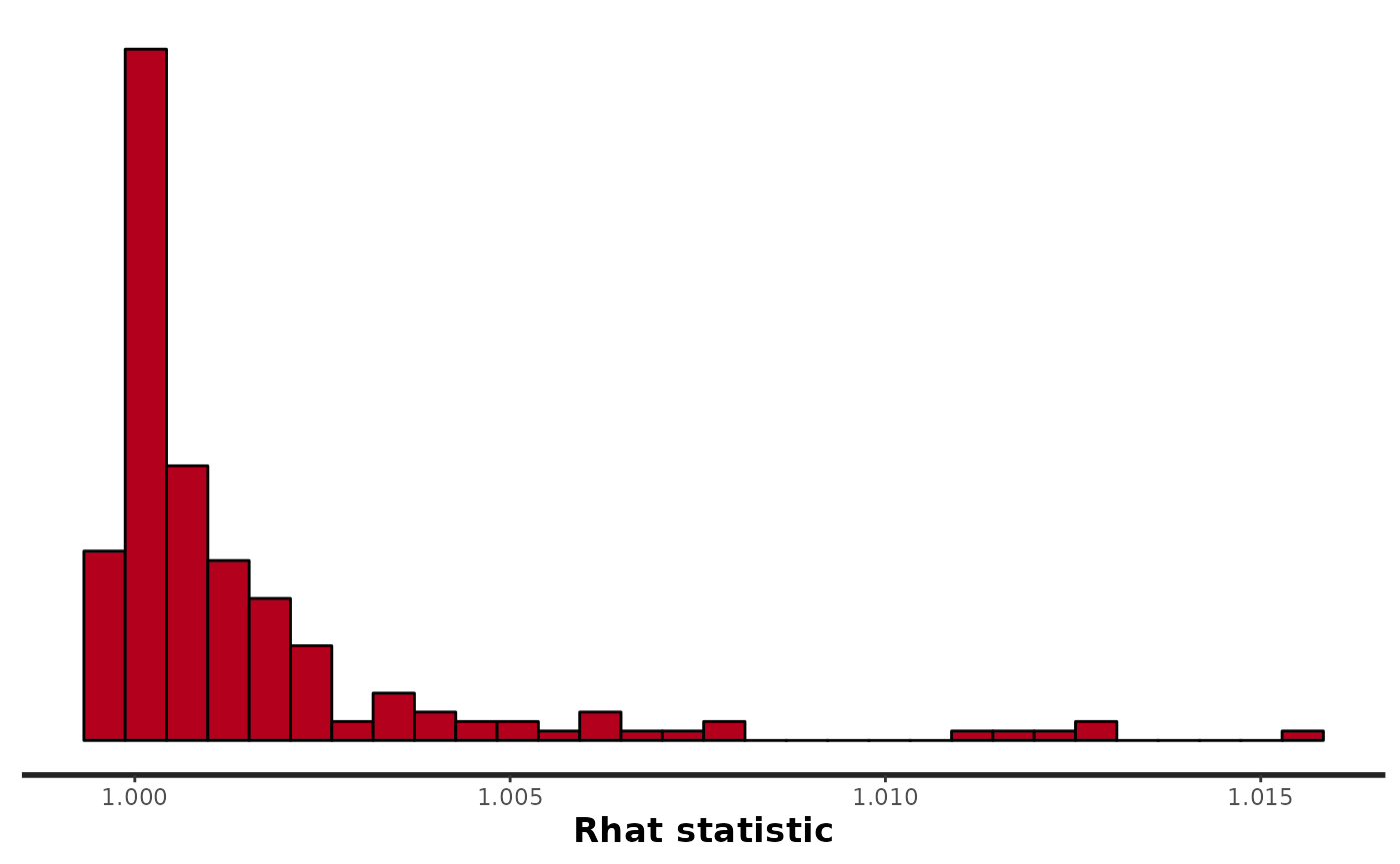
monitor(rstan::extract(fit, pars = params, permuted = FALSE, inc_warmup = TRUE))
#> Inference for the input samples (4 chains: each with iter = 5000; warmup = 2500):
#>
#>            Q5   Q50   Q95  Mean   SD  Rhat Bulk_ESS Tail_ESS
#> Sopt[1]   0.3   0.5   0.7   0.5  0.1  1.00     3230     2104
#> Sopt[2]   0.4   1.1   1.9   1.1  0.5  1.00     3572     2468
#> Sopt[3]   2.1   2.8 136.6  18.2 42.2  1.01      674     1084
#> Sopt[4]   1.1  56.3 184.0  69.5 64.9  1.00     1109     3902
#> Sopt[5]   5.9  84.4 187.3  88.8 60.0  1.00     3074     2002
#> Sopt[6]   7.4  95.9 189.6  97.3 58.7  1.00     6825     4102
#> Sopt[7]   2.3  20.9 180.4  55.0 62.2  1.00     1748     5784
#> Sopt[8]   0.8   1.2  39.0   7.4 27.7  1.00     1693      795
#> Sopt[9]   6.2   8.3  14.7   9.9 10.1  1.00     4348     1993
#> Sopt[10]  2.6   9.9 176.8  47.6 59.9  1.00     1758     5542
#> Sopt[11] 10.6  93.6 189.1  95.6 58.3  1.00     5489     4772
#> Sopt[12] 14.5 102.1 189.8 101.7 56.6  1.00     7631     6317
#> Sopt[13] 28.6 103.3 189.7 105.6 52.0  1.00     4054     4542
#> hopt[1]   0.1   0.3   0.5   0.3  0.1  1.00     3257     2187
#> hopt[2]   0.0   0.1   0.3   0.1  0.1  1.00     3831     2456
#> hopt[3]   0.0   0.4   0.6   0.4  0.2  1.01      613     1060
#> hopt[4]   0.1   0.3   0.7   0.3  0.2  1.00     1050     3301
#> hopt[5]   0.4   0.5   0.7   0.5  0.1  1.00     3663     1792
#> hopt[6]   0.2   0.3   0.4   0.3  0.1  1.00     7582     4514
#> hopt[7]   0.5   0.6   0.8   0.6  0.1  1.00     1833     5191
#> hopt[8]   0.6   0.8   0.8   0.7  0.1  1.00     1764      985
#> hopt[9]   0.7   0.8   0.9   0.8  0.1  1.00     4725     2291
#> hopt[10]  0.2   0.4   0.6   0.4  0.1  1.00     1766     5338
#> hopt[11]  0.0   0.2   0.4   0.2  0.1  1.00     3992     2883
#> hopt[12]  0.3   0.4   0.5   0.4  0.1  1.00     8919     6485
#> hopt[13]  0.5   0.6   0.7   0.6  0.1  1.00     5358     3892
#> tau       2.8   3.7   4.7   3.7  0.6  1.01     1225     2927
#>
#> For each parameter, Bulk_ESS and Tail_ESS are crude measures of
#> effective sample size for bulk and tail quantities respectively (an ESS > 100
#> per chain is considered good), and Rhat is the potential scale reduction
#> factor on rank normalized split chains (at convergence, Rhat <= 1.05).
print(fit, par = c("lp__", params) )
#> Inference for Stan model: HSR_Ricker_LogN_Management.
#> 4 chains, each with iter=5000; warmup=2500; thin=1;
#> post-warmup draws per chain=2500, total post-warmup draws=10000.
#>
#>            mean se_mean    sd  2.5%   25%    50%    75%  97.5% n_eff Rhat
#> lp__      26.21    0.22  5.38 14.33 22.77  26.61  30.14  35.40   623 1.01
#> Sopt[1]    0.51    0.00  0.12  0.22  0.44   0.53   0.59   0.71  2631 1.00
#> Sopt[2]    1.11    0.01  0.46  0.24  0.78   1.11   1.43   1.99  3693 1.00
#> Sopt[3]   18.23    2.08 42.23  1.99  2.51   2.84   3.52 168.77   412 1.02
#> Sopt[4]   69.47    1.74 64.93  1.06  2.52  56.25 125.33 192.80  1390 1.00
#> Sopt[5]   88.80    0.93 60.05  4.65 32.68  84.36 140.52 193.90  4161 1.00
#> Sopt[6]   97.25    0.64 58.73  3.45 45.79  95.94 148.59 194.98  8301 1.00
#> Sopt[7]   55.04    1.31 62.22  2.09  3.68  20.86 103.51 190.79  2249 1.00
#> Sopt[8]    7.43    0.96 27.68  0.81  1.00   1.16   1.45 116.59   830 1.00
#> Sopt[9]    9.87    0.32 10.06  5.96  7.27   8.29   9.81  19.59   965 1.00
#> Sopt[10]  47.64    1.31 59.91  2.48  3.62   9.86  84.24 188.54  2087 1.00
#> Sopt[11]  95.63    0.73 58.29  8.17 42.54  93.65 145.98 194.77  6334 1.00
#> Sopt[12] 101.75    0.61 56.65  9.70 51.97 102.13 150.95 194.63  8597 1.00
#> Sopt[13] 105.57    0.77 51.99 23.91 59.75 103.31 150.03 194.79  4586 1.00
#> hopt[1]    0.31    0.00  0.13  0.08  0.22   0.31   0.40   0.56  3500 1.00
#> hopt[2]    0.15    0.00  0.08  0.02  0.09   0.14   0.20   0.33  4823 1.00
#> hopt[3]    0.35    0.01  0.16  0.02  0.25   0.38   0.47   0.61   465 1.01
#> hopt[4]    0.32    0.01  0.17  0.08  0.20   0.27   0.39   0.73   841 1.00
#> hopt[5]    0.48    0.00  0.09  0.35  0.43   0.47   0.52   0.73  2251 1.00
#> hopt[6]    0.31    0.00  0.09  0.14  0.25   0.31   0.36   0.48  6493 1.00
#> hopt[7]    0.63    0.00  0.10  0.47  0.55   0.60   0.71   0.83  1603 1.00
#> hopt[8]    0.75    0.00  0.08  0.52  0.71   0.76   0.80   0.86  1003 1.00
#> hopt[9]    0.80    0.00  0.06  0.65  0.77   0.81   0.84   0.89  3000 1.00
#> hopt[10]   0.38    0.00  0.14  0.16  0.28   0.36   0.49   0.65  1611 1.00
#> hopt[11]   0.20    0.00  0.12  0.02  0.12   0.18   0.26   0.50  4151 1.00
#> hopt[12]   0.43    0.00  0.07  0.28  0.38   0.43   0.48   0.57  8462 1.00
#> hopt[13]   0.58    0.00  0.08  0.44  0.52   0.57   0.62   0.78  4580 1.00
#> tau        3.73    0.02  0.57  2.69  3.33   3.71   4.10   4.92  1232 1.01
#>
#> Samples were drawn using NUTS(diag_e) at Mon Aug 29 19:55:21 2022.
#> For each parameter, n_eff is a crude measure of effective sample size,
#> and Rhat is the potential scale reduction factor on split chains (at
#> convergence, Rhat=1).
dfw_unif <- extract_wider(fit)
dfl_unif <- extract_longer(fit)

dfl_unif %>%
  filter(str_detect(parameter, "Sopt")) %>%
  mutate(Site = SRSalmon$name_riv[as.integer(str_sub(parameter, str_length("Sopt.") + 1))]) %>%
  ggplot(aes(y = log(value), x = Site)) +
  geom_boxplot(fill = "grey80") +
  ylab("log(S*)") +
  plot_theme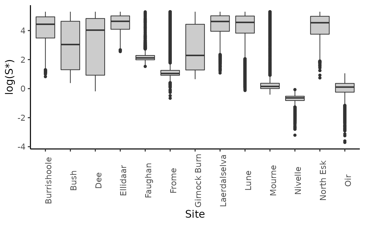
dfl_unif %>%
  filter(str_detect(parameter, "hopt")) %>%
  mutate(Site = SRSalmon$name_riv[as.integer(str_sub(parameter, str_length("hopt.") + 1))]) %>%
  ggplot(aes(y = log(value), x = Site)) +
  geom_boxplot(fill = "grey80") +
  ylab("log(h*)") +
  plot_theme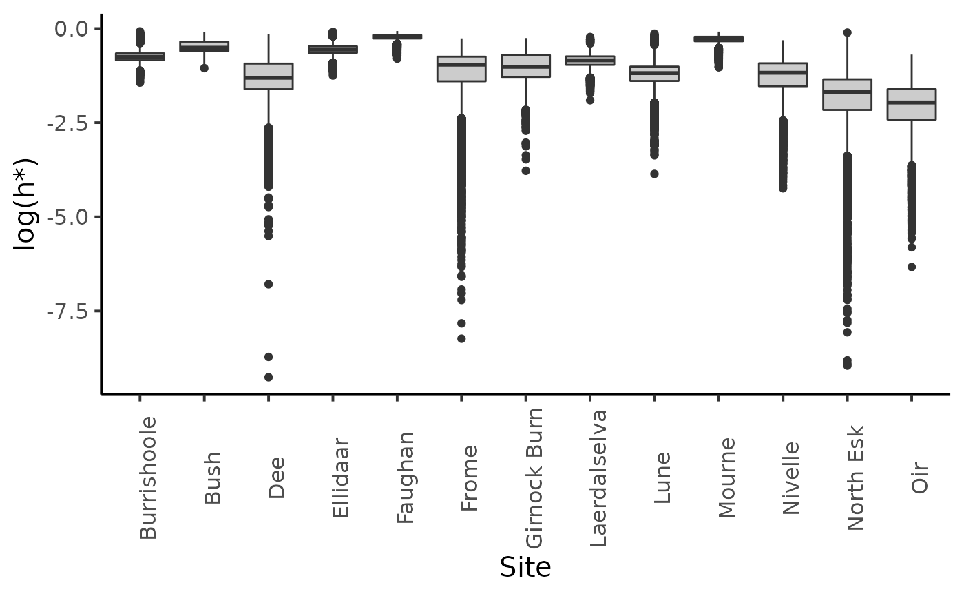
Model with no covariates and with Gamma prior for \(S*\)
hsr_model_indep_S_gamma_stan <- "
data {
  int n_riv; // Number of rivers
  int n_obs[n_riv]; // Number of observations by rivers
  int n; // Total number of observations
  int riv[n]; // River membership (indices k)
  vector[n] S; // Stock data
  vector[n] R; // Recruitment data
}

parameters {
  vector<lower=0, upper=200>[n_riv] Sopt;
  vector<lower=0, upper=1>[n_riv] hopt;
  real<lower=0> tau;
}

transformed parameters {
  vector<lower=0>[n_riv] alpha;
  vector<lower=0>[n_riv] beta ;
  real<lower=0> sigma;
  // real Copt;
  // real Ropt;
  vector[n] LogR;
  // real Slope;

  for (k in 1:n_riv) {
    alpha[k] = exp(hopt[k])/(1-hopt[k]) ;
    beta[k] = hopt[k]/Sopt[k]     ;
  }
  sigma = tau^-0.5        ;
  // Copt = hopt*Sopt/(1-hopt);
  // Ropt = Sopt + Copt;
  // Slope = exp(alpha);
  for (t in 1:n) {
    LogR[t] = log(S[t]) + log(alpha[riv[t]]) - beta[riv[t]]*S[t] ;  // LogR[t] is the logarithm of the Ricker function
  }
}

model {
  tau ~ gamma(.001, .001) ; // Diffuse prior for the variance
  for (k in 1:n_riv) {
    hopt[k] ~ beta(1,1) ;
    Sopt[k] ~ gamma(1, 1./1600) ;
  }
//
    log(R) ~ normal(LogR, sigma) ;
}
"
model_name <-"HSR_Ricker_LogN_Management_S_gamma"
sm <- stan_model(model_code =  hsr_model_indep_S_gamma_stan,
                 model_name =  model_name
)
#> Running /usr/lib/R/bin/R CMD SHLIB foo.c
#> gcc -I"/usr/share/R/include" -DNDEBUG   -I"/home/chabertliddell/R/x86_64-pc-linux-gnu-library/4.2/Rcpp/include/"  -I"/home/chabertliddell/R/x86_64-pc-linux-gnu-library/4.2/RcppEigen/include/"  -I"/home/chabertliddell/R/x86_64-pc-linux-gnu-library/4.2/RcppEigen/include/unsupported"  -I"/home/chabertliddell/R/x86_64-pc-linux-gnu-library/4.2/BH/include" -I"/home/chabertliddell/R/x86_64-pc-linux-gnu-library/4.2/StanHeaders/include/src/"  -I"/home/chabertliddell/R/x86_64-pc-linux-gnu-library/4.2/StanHeaders/include/"  -I"/home/chabertliddell/R/x86_64-pc-linux-gnu-library/4.2/RcppParallel/include/"  -I"/home/chabertliddell/R/x86_64-pc-linux-gnu-library/4.2/rstan/include" -DEIGEN_NO_DEBUG  -DBOOST_DISABLE_ASSERTS  -DBOOST_PENDING_INTEGER_LOG2_HPP  -DSTAN_THREADS  -DBOOST_NO_AUTO_PTR  -include '/home/chabertliddell/R/x86_64-pc-linux-gnu-library/4.2/StanHeaders/include/stan/math/prim/mat/fun/Eigen.hpp'  -D_REENTRANT -DRCPP_PARALLEL_USE_TBB=1      -fpic  -g -O2 -fdebug-prefix-map=/build/r-base-zYgbYq/r-base-4.2.1=. -fstack-protector-strong -Wformat -Werror=format-security -Wdate-time -D_FORTIFY_SOURCE=2  -c foo.c -o foo.o
#> In file included from /home/chabertliddell/R/x86_64-pc-linux-gnu-library/4.2/RcppEigen/include/Eigen/Core:88,
#>                  from /home/chabertliddell/R/x86_64-pc-linux-gnu-library/4.2/RcppEigen/include/Eigen/Dense:1,
#>                  from /home/chabertliddell/R/x86_64-pc-linux-gnu-library/4.2/StanHeaders/include/stan/math/prim/mat/fun/Eigen.hpp:13,
#>                  from <command-line>:
#> /home/chabertliddell/R/x86_64-pc-linux-gnu-library/4.2/RcppEigen/include/Eigen/src/Core/util/Macros.h:628:1: error: unknown type name ‘namespace’
#>   628 | namespace Eigen {
#>       | ^~~~~~~~~
#> /home/chabertliddell/R/x86_64-pc-linux-gnu-library/4.2/RcppEigen/include/Eigen/src/Core/util/Macros.h:628:17: error: expected ‘=’, ‘,’, ‘;’, ‘asm’ or ‘__attribute__’ before ‘{’ token
#>   628 | namespace Eigen {
#>       |                 ^
#> In file included from /home/chabertliddell/R/x86_64-pc-linux-gnu-library/4.2/RcppEigen/include/Eigen/Dense:1,
#>                  from /home/chabertliddell/R/x86_64-pc-linux-gnu-library/4.2/StanHeaders/include/stan/math/prim/mat/fun/Eigen.hpp:13,
#>                  from <command-line>:
#> /home/chabertliddell/R/x86_64-pc-linux-gnu-library/4.2/RcppEigen/include/Eigen/Core:96:10: fatal error: complex: No such file or directory
#>    96 | #include <complex>
#>       |          ^~~~~~~~~
#> compilation terminated.
#> make: *** [/usr/lib/R/etc/Makeconf:168: foo.o] Error 1
set.seed(1234)
# Number iteration for the "warm up" phase
n_warm <- 2500
# Number iteration for inferences
n_iter <- 5000
n_thin <- 1
# Number of chains
n_chains <- 4

params<-c("Sopt","hopt","tau")
# Inferences


fit <- sampling(object = sm,
                data = SRSalmon,
                pars = NA, #params,
                chains = n_chains,
                iter = n_iter,
                warmup = n_warm,
                thin = n_thin,
                control = list("adapt_delta" = .85)# Acceptance rate up from .8 to remove some divergent transitions
)
Diagnostic of the convergence:
params<-c("Sopt","hopt","tau")
stan_rhat(fit)
#> `stat_bin()` using `bins = 30`. Pick better value with `binwidth`.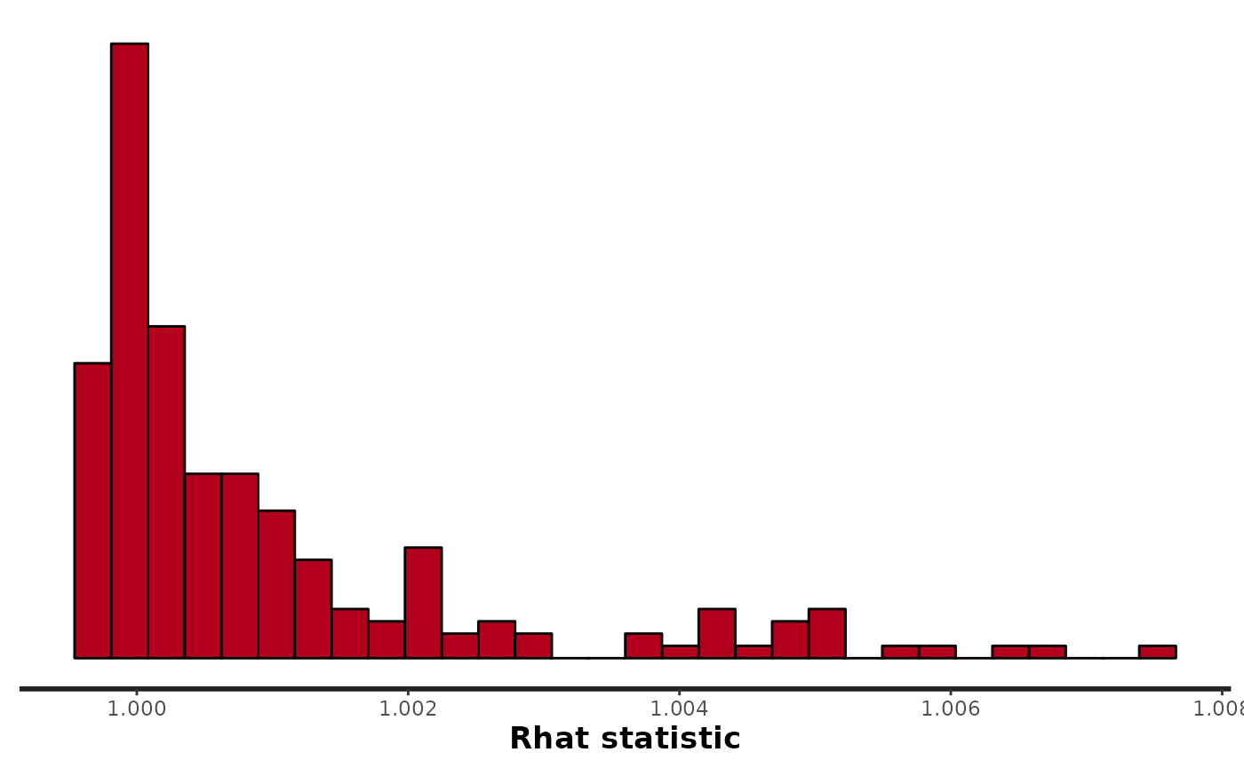
monitor(rstan::extract(fit, pars = params, permuted = FALSE, inc_warmup = TRUE))
#> Inference for the input samples (4 chains: each with iter = 5000; warmup = 2500):
#>
#>            Q5   Q50   Q95  Mean   SD  Rhat Bulk_ESS Tail_ESS
#> Sopt[1]   0.3   0.5   0.7   0.5  0.1  1.00     3281     1910
#> Sopt[2]   0.4   1.1   1.9   1.1  0.4  1.00     3864     2874
#> Sopt[3]   2.1   2.8 123.8  16.3 39.1  1.00      906     1235
#> Sopt[4]   1.1  48.9 183.7  66.6 64.6  1.00     1257     4396
#> Sopt[5]   5.9  78.5 187.0  85.1 60.0  1.00     3312     2234
#> Sopt[6]   6.7  92.5 188.8  95.1 58.8  1.00     6604     3476
#> Sopt[7]   2.2  18.2 176.7  52.4 60.5  1.00     1976     5773
#> Sopt[8]   0.8   1.2  44.3   7.6 27.8  1.00     1548      648
#> Sopt[9]   6.2   8.3  14.0   9.1  3.9  1.00     4717     3206
#> Sopt[10]  2.7   8.6 173.9  45.9 58.6  1.00     1736     6340
#> Sopt[11] 10.3  87.7 187.7  91.9 59.0  1.00     6135     5340
#> Sopt[12] 14.8  97.9 190.2 100.0 56.6  1.00     6915     5028
#> Sopt[13] 27.4 100.0 189.2 103.6 52.0  1.00     3616     3879
#> hopt[1]   0.1   0.3   0.5   0.3  0.1  1.00     3112     1735
#> hopt[2]   0.0   0.1   0.3   0.2  0.1  1.00     3997     2839
#> hopt[3]   0.0   0.4   0.6   0.4  0.2  1.01      789      978
#> hopt[4]   0.1   0.3   0.7   0.3  0.2  1.00     1235     4129
#> hopt[5]   0.4   0.5   0.7   0.5  0.1  1.00     4065     2135
#> hopt[6]   0.2   0.3   0.5   0.3  0.1  1.00     6894     4684
#> hopt[7]   0.5   0.6   0.8   0.6  0.1  1.00     2054     5313
#> hopt[8]   0.6   0.8   0.8   0.7  0.1  1.00     1601      762
#> hopt[9]   0.7   0.8   0.9   0.8  0.1  1.00     4764     3686
#> hopt[10]  0.2   0.4   0.6   0.4  0.1  1.00     1697     4804
#> hopt[11]  0.0   0.2   0.4   0.2  0.1  1.00     5131     3521
#> hopt[12]  0.3   0.4   0.5   0.4  0.1  1.00     8140     5414
#> hopt[13]  0.5   0.6   0.7   0.6  0.1  1.00     5063     3527
#> tau       2.9   3.7   4.7   3.7  0.6  1.00     1499     3492
#>
#> For each parameter, Bulk_ESS and Tail_ESS are crude measures of
#> effective sample size for bulk and tail quantities respectively (an ESS > 100
#> per chain is considered good), and Rhat is the potential scale reduction
#> factor on rank normalized split chains (at convergence, Rhat <= 1.05).
print(fit, par = c("lp__", params) )
#> Inference for Stan model: HSR_Ricker_LogN_Management_S_gamma.
#> 4 chains, each with iter=5000; warmup=2500; thin=1;
#> post-warmup draws per chain=2500, total post-warmup draws=10000.
#>
#>            mean se_mean    sd  2.5%   25%   50%    75%  97.5% n_eff Rhat
#> lp__      26.02    0.19  5.24 14.73 22.67 26.39  29.74  35.24   778 1.01
#> Sopt[1]    0.51    0.00  0.13  0.21  0.44  0.53   0.60   0.72  2668 1.00
#> Sopt[2]    1.12    0.01  0.45  0.28  0.80  1.12   1.43   1.99  4105 1.00
#> Sopt[3]   16.30    1.64 39.07  2.01  2.51  2.84   3.47 160.48   568 1.01
#> Sopt[4]   66.61    1.62 64.57  1.06  2.18 48.85 121.70 191.90  1591 1.00
#> Sopt[5]   85.15    0.88 60.02  4.53 28.80 78.52 136.63 193.00  4655 1.00
#> Sopt[6]   95.08    0.64 58.82  3.18 43.41 92.51 146.30 194.66  8318 1.00
#> Sopt[7]   52.36    1.21 60.49  2.04  3.61 18.23  96.33 189.11  2496 1.00
#> Sopt[8]    7.57    1.10 27.76  0.81  1.00  1.16   1.45 116.83   637 1.01
#> Sopt[9]    9.11    0.08  3.94  5.94  7.29  8.30   9.80  16.84  2625 1.00
#> Sopt[10]  45.89    1.37 58.65  2.49  3.58  8.59  80.33 187.28  1832 1.00
#> Sopt[11]  91.90    0.70 59.04  8.15 36.32 87.74 143.43 193.71  7048 1.00
#> Sopt[12]  99.96    0.63 56.60  9.76 49.92 97.89 149.17 194.59  8039 1.00
#> Sopt[13] 103.62    0.81 51.97 22.67 58.37 99.98 147.70 194.97  4163 1.00
#> hopt[1]    0.31    0.00  0.13  0.08  0.22  0.31   0.40   0.56  3429 1.00
#> hopt[2]    0.15    0.00  0.08  0.03  0.09  0.14   0.20   0.32  5004 1.00
#> hopt[3]    0.36    0.01  0.16  0.02  0.26  0.39   0.48   0.61   633 1.01
#> hopt[4]    0.32    0.01  0.17  0.09  0.20  0.27   0.41   0.72   944 1.00
#> hopt[5]    0.49    0.00  0.09  0.35  0.43  0.47   0.52   0.73  2598 1.00
#> hopt[6]    0.31    0.00  0.09  0.14  0.25  0.31   0.36   0.49  5487 1.00
#> hopt[7]    0.63    0.00  0.10  0.47  0.55  0.60   0.71   0.83  1800 1.00
#> hopt[8]    0.75    0.00  0.08  0.52  0.71  0.76   0.80   0.86   864 1.01
#> hopt[9]    0.80    0.00  0.06  0.66  0.77  0.81   0.84   0.89  4043 1.00
#> hopt[10]   0.39    0.00  0.14  0.16  0.28  0.37   0.50   0.65  1556 1.00
#> hopt[11]   0.21    0.00  0.12  0.02  0.12  0.19   0.27   0.52  5260 1.00
#> hopt[12]   0.43    0.00  0.08  0.28  0.38  0.43   0.48   0.57  7608 1.00
#> hopt[13]   0.58    0.00  0.08  0.44  0.53  0.57   0.63   0.79  4246 1.00
#> tau        3.74    0.01  0.57  2.71  3.34  3.71   4.11   4.93  1477 1.00
#>
#> Samples were drawn using NUTS(diag_e) at Mon Aug 29 19:56:14 2022.
#> For each parameter, n_eff is a crude measure of effective sample size,
#> and Rhat is the potential scale reduction factor on split chains (at
#> convergence, Rhat=1).
dfw_gamma <- extract_wider(fit) %>% mutate(Model = "Gamma")
dfl_gamma <- extract_longer(fit)

dfl_gamma %>%
  filter(str_detect(parameter, "Sopt")) %>%
  mutate(Site = SRSalmon$name_riv[as.integer(str_sub(parameter, str_length("Sopt.") + 1))]) %>%
  ggplot(aes(y = log(value), x = Site)) +
  geom_boxplot(fill = "grey80") +
  ylab("log(S*)") +
  plot_theme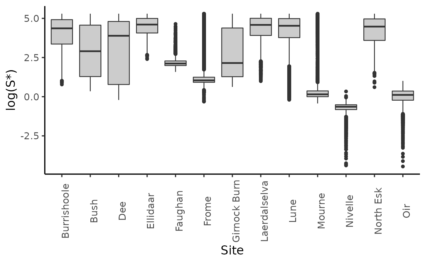
dfl_gamma %>%
  filter(str_detect(parameter, "hopt")) %>%
  mutate(Site = SRSalmon$name_riv[as.integer(str_sub(parameter, str_length("hopt.") + 1))]) %>%
  ggplot(aes(y = log(value), x = Site)) +
  geom_boxplot(fill = "grey80") +
  ylab("log(h*)") +
  plot_theme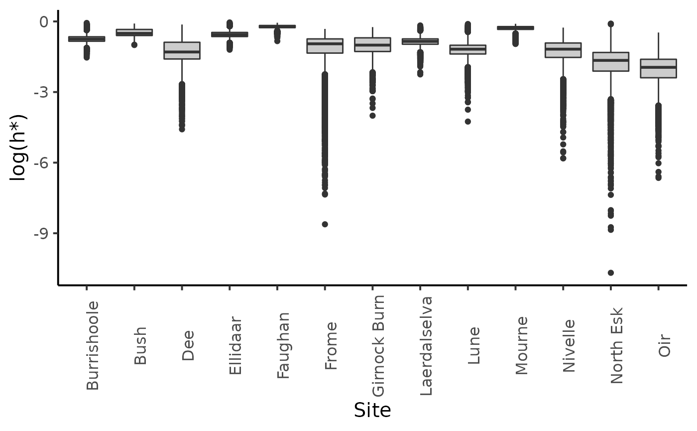
The choice of the prior distribution of \(S^*\) does not make much difference on the posterior distribution estimate.
bind_rows(dfl_unif %>% mutate (Model =  "Uniform"), dfl_gamma %>%  mutate(Model = "Gamma")) %>%
  filter(str_detect(parameter, "Sopt")) %>%
  mutate(Site = SRSalmon$name_riv[as.integer(str_sub(parameter, str_length("Sopt.") + 1))]) %>%
  ggplot(aes(x = log(value), linetype = Model, color = Model)) +
  geom_density() +
  facet_wrap(~ Site) +
  xlab("log(S*)") +
  plot_theme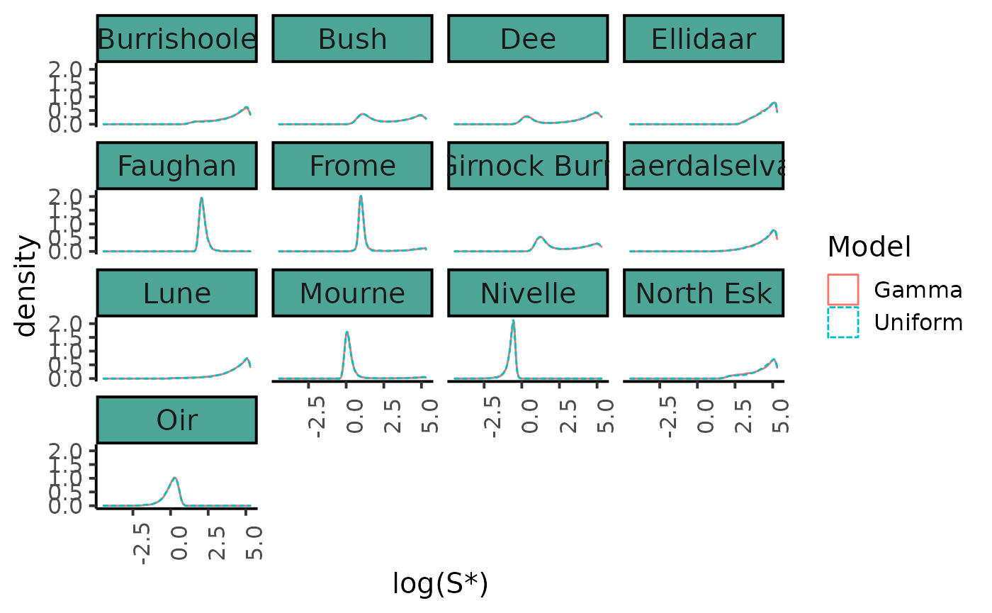
Hierarchical model with latitudinal covariates
The hierarchical modeling is designed to improve the estimation of parameters \(S^*\) and \(h^*\) for data-poor rivers by borrowing strength from data-rich rivers. It is then designed to capture the between-rivers variability of the parameters (\(S^*\), \(h^*\)) conditionnaly on the latitude. This can be done by introducing a log-linear relationship between the expectation of \(S^*_k\) and the latitude of the river \(x_k\):
- \(\log(\mu_{S^*_k}) = \alpha x_k + \beta\)
- \(\alpha \sim Uniform(-5,5)\)
- \(\beta \sim Uniform(-50,50)\)
\(S^*_k\) is drawn from a Gamma distribution which the parameters depend on the latitude:
- \(CV_{S^*} ~ Uniform(0,20)\)
- \(a_k = \frac{1}{CV_{S*}^2}\)
- \(b_k = \frac{1}{\mu_{S^*_k}CV^2_{S^*}}\)
- \(S^*_k \sim Gamma(a_k, b_k)1_{S^*_k<200}\)
Then we express the linear linear relationship between the expectation of \(h^*_k\) and the latitude of the river \(x_k\) on a logit scale:
- \(logit(\mu_{h^*_k}) = \delta x_k + \kappa\)
- \(\delta \sim Uniform(-5,5)\)
- \(\kappa \sim Uniform(-50,50)\)
Given the expected mean in the logit scale, \(logit(h_{k}^{\ast})\) for each river \(k\) is drawn in a Normal distribution with expected mean \(logit(\mu_{h_{k}^{\ast}})\) and precision \(\tau_{h^{\ast}}^{-2}\). A diffuse prior is set on the precision:
- \(logit(h^*_k) \sim Normal(logit(\mu_k^*), \tau^2)\)
- \(\tau^{-2} \sim Gamma(.001, .001)\)
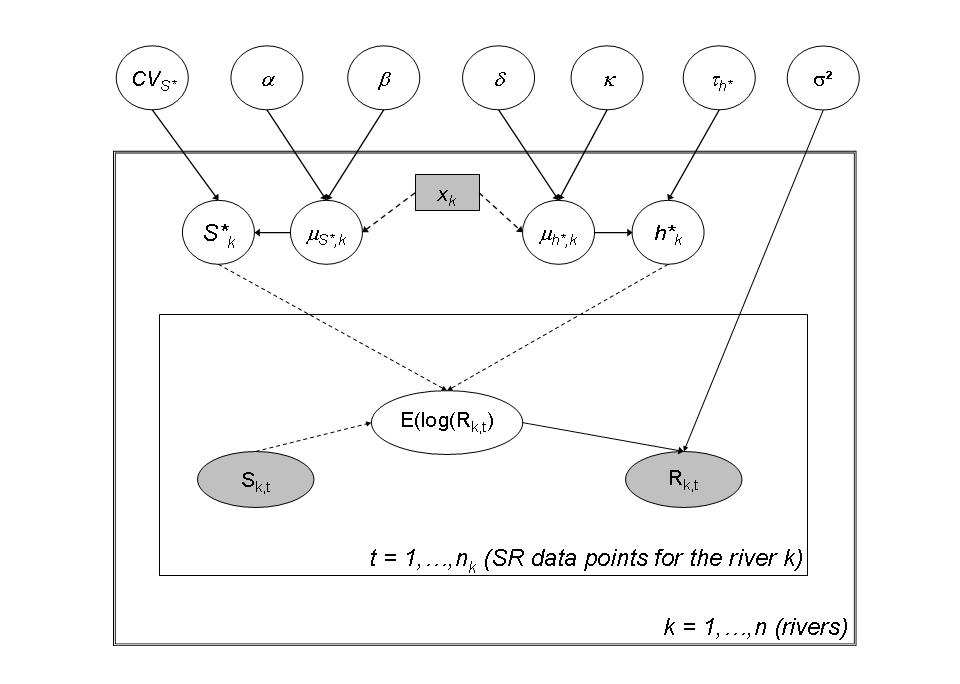
Directed acyclic graph of the stock recruitment model with covariates
hsr_model_hier_S_gamma_stan <- "
data {
  int n_riv; // Number of rivers
  int n_obs[n_riv]; // Number of observations by rivers
  int n; // Total number of observations
  int riv[n]; // River membership (indices k)
  vector<lower=0>[n] S; // Stock data
  vector<lower=0>[n] R; // Recruitment data
  vector[n_riv] lat; //Latitude of rivers
  int n_pred;
  vector[n_pred] lat_pred;
}

transformed data {
  vector[n_riv] lat_rescaled;
//  real CV_S;
//  real a;
//  a = 1/(CV_S*CV_S);
  lat_rescaled = lat-mean(lat);
}

parameters {
  real<lower=0> tau;

  real<lower=0, upper=20> CV_S;
  real<lower=-5, upper=5> alpha;
  real<lower=-50, upper=50> beta;
  vector<lower=0, upper=200>[n_riv] Sopt;


  real<lower=-5, upper=5> delta;
  real<lower=-50, upper=50> kappa;
  real<lower=0> tau_h;
  vector[n_riv] logit_h;
  //vector[n_riv] logit_h_raw; // centered parametrization for logit_h

}

transformed parameters {

  real<lower=0> sigma;      // stdev for lognormal noise

//  vector[n_riv] log_mu_S; // log of the expected mean of Sopt
  vector<lower=0>[n_riv] mu_S; // Expected mean of Sopt
  real<lower=0> a; // parameters of the gamma prior of Sopt
  vector<lower=0>[n_riv] b; // parameters of the gamma prior of Sopt

  real<lower=0> sigma_h; // stdev for logit of h
  vector[n_riv] logit_mu_h; // logit of the expected mean of hopt
  vector<lower=0, upper=1>[n_riv] hopt;

  //vector[n_riv] logit_h;   // logit of hopt
  vector[n] LogR;


  sigma = tau^-0.5  ;
  sigma_h = tau_h^-0.5 ;

  for (k in 1:n_riv) {
    mu_S[k] = exp(alpha * (lat[k]) + beta) ;
//    mu_S[k] = exp(alpha * (lat_rescaled[k]) + beta) ;
//    mu_S[k] = exp(log_mu_S[k]);
    logit_mu_h[k] = delta * (lat[k]) + kappa ;
//    logit_mu_h[k] = delta * (lat_rescaled[k]) + kappa ;
   // logit_h[k] = logit_mu_h[k] + sigma_h * logit_h_raw[k];
  }

  a = 1/square(CV_S) ;
  for (k in 1:n_riv) {
    b[k] = 1/(mu_S[k]*square(CV_S)) ;
  }
  hopt = inv_logit(logit_h) ;


  for (t in 1:n) {
    LogR[t] = hopt[riv[t]] + log(S[t]) - log(1 - hopt[riv[t]]) - hopt[riv[t]]/Sopt[riv[t]]*S[t] ;  // LogR[t] is the logarithm of the Ricker function
  }
}

model {
//  alpha ~ uniform(-5, 5);
//  beta ~ uniform(-50, 50);
//  CV_S ~ uniform(0, 20);

//  delta ~ uniform(-5, 5);
//  kappa ~ uniform(-50, 50);


  tau ~ gamma(.001, .001) ; // Diffuse prior for the precision
  tau_h ~ gamma(.001, .001) ; // Diffuse prior for the precision


  //logit_h_raw ~ std_normal();
  for (k in 1:n_riv) {
    logit_h[k] ~ normal(logit_mu_h[k], sigma_h);
    Sopt[k] ~ gamma(a, b[k]) ; // T[0,200] ;
  }


  log(R) ~ normal(LogR, sigma) ;
}

generated quantities {
  real a_pred;
  vector[n_pred] b_pred;
  vector[n_pred] Sopt_pred;
  vector[n_pred] logit_hopt_pred;
  vector<lower=0,upper=1>[n_pred] hopt_pred;
  // Posterior Predictive for new rivers with latitude lat_pred[p]
  a_pred = 1/(CV_S*CV_S);
  for ( p in 1 : n_pred ) {
//    b_pred[p] = a/(exp(alpha * lat_pred[p] + beta - alpha * mean(lat)));
    b_pred[p] = a_pred*(1/exp(alpha * lat_pred[p] + beta));
    Sopt_pred[p] = gamma_rng(a_pred,b_pred[p]); //T[0,200];
//    logit_hopt_pred[p] = normal_rng(exp(delta * lat_pred[p] + kappa - delta * mean(lat)), sigma_h);`
    logit_hopt_pred[p] = normal_rng(delta * lat_pred[p] + kappa, sigma_h);
    hopt_pred[p] = inv_logit(logit_hopt_pred[p]);
  } // end loop on predictions p
}
"
model_name_hier <-"HSR_Ricker_LogN_Management_S_gamma_hier"
sm_hier <- stan_model(model_code =  hsr_model_hier_S_gamma_stan,
                 model_name =  model_name_hier)
#> Trying to compile a simple C file
#> Running /usr/lib/R/bin/R CMD SHLIB foo.c
#> gcc -I"/usr/share/R/include" -DNDEBUG   -I"/home/chabertliddell/R/x86_64-pc-linux-gnu-library/4.2/Rcpp/include/"  -I"/home/chabertliddell/R/x86_64-pc-linux-gnu-library/4.2/RcppEigen/include/"  -I"/home/chabertliddell/R/x86_64-pc-linux-gnu-library/4.2/RcppEigen/include/unsupported"  -I"/home/chabertliddell/R/x86_64-pc-linux-gnu-library/4.2/BH/include" -I"/home/chabertliddell/R/x86_64-pc-linux-gnu-library/4.2/StanHeaders/include/src/"  -I"/home/chabertliddell/R/x86_64-pc-linux-gnu-library/4.2/StanHeaders/include/"  -I"/home/chabertliddell/R/x86_64-pc-linux-gnu-library/4.2/RcppParallel/include/"  -I"/home/chabertliddell/R/x86_64-pc-linux-gnu-library/4.2/rstan/include" -DEIGEN_NO_DEBUG  -DBOOST_DISABLE_ASSERTS  -DBOOST_PENDING_INTEGER_LOG2_HPP  -DSTAN_THREADS  -DBOOST_NO_AUTO_PTR  -include '/home/chabertliddell/R/x86_64-pc-linux-gnu-library/4.2/StanHeaders/include/stan/math/prim/mat/fun/Eigen.hpp'  -D_REENTRANT -DRCPP_PARALLEL_USE_TBB=1      -fpic  -g -O2 -fdebug-prefix-map=/build/r-base-zYgbYq/r-base-4.2.1=. -fstack-protector-strong -Wformat -Werror=format-security -Wdate-time -D_FORTIFY_SOURCE=2  -c foo.c -o foo.o
#> In file included from /home/chabertliddell/R/x86_64-pc-linux-gnu-library/4.2/RcppEigen/include/Eigen/Core:88,
#>                  from /home/chabertliddell/R/x86_64-pc-linux-gnu-library/4.2/RcppEigen/include/Eigen/Dense:1,
#>                  from /home/chabertliddell/R/x86_64-pc-linux-gnu-library/4.2/StanHeaders/include/stan/math/prim/mat/fun/Eigen.hpp:13,
#>                  from <command-line>:
#> /home/chabertliddell/R/x86_64-pc-linux-gnu-library/4.2/RcppEigen/include/Eigen/src/Core/util/Macros.h:628:1: error: unknown type name ‘namespace’
#>   628 | namespace Eigen {
#>       | ^~~~~~~~~
#> /home/chabertliddell/R/x86_64-pc-linux-gnu-library/4.2/RcppEigen/include/Eigen/src/Core/util/Macros.h:628:17: error: expected ‘=’, ‘,’, ‘;’, ‘asm’ or ‘__attribute__’ before ‘{’ token
#>   628 | namespace Eigen {
#>       |                 ^
#> In file included from /home/chabertliddell/R/x86_64-pc-linux-gnu-library/4.2/RcppEigen/include/Eigen/Dense:1,
#>                  from /home/chabertliddell/R/x86_64-pc-linux-gnu-library/4.2/StanHeaders/include/stan/math/prim/mat/fun/Eigen.hpp:13,
#>                  from <command-line>:
#> /home/chabertliddell/R/x86_64-pc-linux-gnu-library/4.2/RcppEigen/include/Eigen/Core:96:10: fatal error: complex: No such file or directory
#>    96 | #include <complex>
#>       |          ^~~~~~~~~
#> compilation terminated.
#> make: *** [/usr/lib/R/etc/Makeconf:168: foo.o] Error 1
# Inferences
set.seed(1234)

fit_hier <- sampling(object = sm_hier,
                data = SRSalmon,
                pars = NA, #params,
                chains = n_chains,
                # init = lapply(seq(4), function(x)
                #   list(alpha = 0, beta = 0)),
                iter = 5000,
                warmup = 2500,
                thin = 1,
                control = list("adapt_delta"= .9)#list("max_treedepth" = 12)
)
#> Warning: There were 9 divergent transitions after warmup. See
#> https://mc-stan.org/misc/warnings.html#divergent-transitions-after-warmup
#> to find out why this is a problem and how to eliminate them.
#> Warning: Examine the pairs() plot to diagnose sampling problems
Diagnostic of the convergence:
params<-c("Sopt","hopt","tau", "delta", "kappa", "alpha", "beta", "CV_S")
stan_rhat(fit_hier)
#> `stat_bin()` using `bins = 30`. Pick better value with `binwidth`.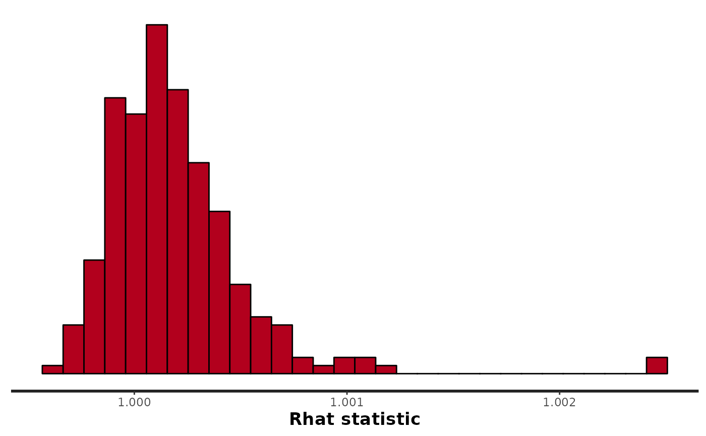
monitor(rstan::extract(fit_hier, pars = params, permuted = FALSE, inc_warmup = TRUE))
#> Inference for the input samples (4 chains: each with iter = 5000; warmup = 2500):
#>
#>             Q5  Q50  Q95 Mean   SD  Rhat Bulk_ESS Tail_ESS
#> Sopt[1]    0.2  0.5  0.6  0.5  0.1     1     4256     2935
#> Sopt[2]    0.6  1.2  1.8  1.2  0.4     1     4341     4047
#> Sopt[3]    2.1  2.6  3.3  2.6  0.4     1     5804     4068
#> Sopt[4]    1.1  1.5  3.3  1.7  1.0     1     5180     3944
#> Sopt[5]    3.3  5.2 10.5  5.9  3.0     1     5419     4681
#> Sopt[6]    1.2  3.0  9.3  3.9  3.1     1     5324     6395
#> Sopt[7]    2.1  3.3  7.3  3.8  2.5     1     5063     4112
#> Sopt[8]    0.9  1.2  2.7  1.5  0.8     1     4747     3120
#> Sopt[9]    6.1  7.7 10.7  8.0  1.5     1     5767     5021
#> Sopt[10]   2.5  3.4  7.2  4.0  2.1     1     5353     3511
#> Sopt[11]   5.8  8.3 16.6  9.4  4.2     1     5665     4375
#> Sopt[12]   4.5 13.2 47.6 18.2 17.3     1     4051     4738
#> Sopt[13]  17.2 30.9 93.0 39.7 27.5     1     3340     2917
#> hopt[1]    0.1  0.3  0.5  0.3  0.1     1     4185     3098
#> hopt[2]    0.1  0.2  0.3  0.2  0.1     1     4284     4059
#> hopt[3]    0.2  0.4  0.6  0.4  0.1     1     6830     3991
#> hopt[4]    0.3  0.5  0.7  0.5  0.1     1     5432     5198
#> hopt[5]    0.5  0.7  0.8  0.7  0.1     1     5973     6012
#> hopt[6]    0.3  0.4  0.7  0.5  0.1     1     5260     5835
#> hopt[7]    0.6  0.7  0.8  0.7  0.1     1     5217     5781
#> hopt[8]    0.6  0.7  0.8  0.7  0.1     1     5035     3944
#> hopt[9]    0.7  0.8  0.9  0.8  0.0     1     5761     6107
#> hopt[10]   0.4  0.5  0.7  0.5  0.1     1     5354     4506
#> hopt[11]   0.2  0.5  0.8  0.5  0.2     1     4564     4443
#> hopt[12]   0.4  0.5  0.7  0.5  0.1     1     5287     5337
#> hopt[13]   0.5  0.7  0.9  0.7  0.1     1     3763     5070
#> tau        3.4  4.3  5.4  4.4  0.6     1     6141     6228
#> delta      0.0  0.1  0.2  0.1  0.1     1     4251     4231
#> kappa    -12.0 -5.7 -0.3 -5.8  3.7     1     4239     4093
#> alpha      0.1  0.2  0.3  0.2  0.0     1     3099     3126
#> beta     -14.2 -9.5 -5.6 -9.7  2.7     1     3180     3281
#> CV_S       0.4  0.6  1.0  0.6  0.2     1     3842     4560
#>
#> For each parameter, Bulk_ESS and Tail_ESS are crude measures of
#> effective sample size for bulk and tail quantities respectively (an ESS > 100
#> per chain is considered good), and Rhat is the potential scale reduction
#> factor on rank normalized split chains (at convergence, Rhat <= 1.05).
print(fit_hier, par = c("lp__", params) )
#> Inference for Stan model: HSR_Ricker_LogN_Management_S_gamma_hier.
#> 4 chains, each with iter=5000; warmup=2500; thin=1;
#> post-warmup draws per chain=2500, total post-warmup draws=10000.
#>
#>           mean se_mean    sd   2.5%    25%   50%   75%  97.5% n_eff Rhat
#> lp__     21.89    0.13  5.62   9.58  18.39 22.47 25.90  31.36  2020    1
#> Sopt[1]   0.45    0.00  0.13   0.16   0.37  0.47  0.55   0.67  3742    1
#> Sopt[2]   1.20    0.01  0.38   0.45   0.93  1.21  1.47   1.93  4315    1
#> Sopt[3]   2.62    0.01  0.40   1.93   2.38  2.59  2.83   3.49  4812    1
#> Sopt[4]   1.74    0.02  0.96   1.01   1.25  1.46  1.86   4.23  3203    1
#> Sopt[5]   5.86    0.05  2.95   3.09   4.20  5.18  6.65  12.58  3727    1
#> Sopt[6]   3.88    0.04  3.13   1.11   1.95  3.01  4.80  11.69  4963    1
#> Sopt[7]   3.85    0.05  2.50   2.01   2.68  3.30  4.25   8.98  3003    1
#> Sopt[8]   1.45    0.02  0.84   0.86   1.06  1.24  1.53   3.57  2584    1
#> Sopt[9]   8.01    0.02  1.53   5.91   7.00  7.74  8.70  11.57  4603    1
#> Sopt[10]  3.99    0.04  2.13   2.40   2.96  3.44  4.26   8.95  2344    1
#> Sopt[11]  9.41    0.07  4.20   5.48   7.03  8.30 10.39  20.41  3645    1
#> Sopt[12] 18.21    0.30 17.26   3.88   8.04 13.15 21.93  64.00  3370    1
#> Sopt[13] 39.72    0.56 27.51  15.77  23.28 30.95 45.02 123.13  2383    1
#> hopt[1]   0.26    0.00  0.12   0.05   0.17  0.25  0.34   0.50  4639    1
#> hopt[2]   0.17    0.00  0.07   0.05   0.12  0.16  0.22   0.33  4750    1
#> hopt[3]   0.42    0.00  0.11   0.19   0.35  0.43  0.49   0.61  6030    1
#> hopt[4]   0.53    0.00  0.13   0.27   0.45  0.54  0.62   0.75  4901    1
#> hopt[5]   0.68    0.00  0.09   0.50   0.62  0.68  0.74   0.85  5926    1
#> hopt[6]   0.46    0.00  0.13   0.24   0.37  0.45  0.54   0.74  5089    1
#> hopt[7]   0.72    0.00  0.07   0.59   0.68  0.72  0.77   0.84  4989    1
#> hopt[8]   0.74    0.00  0.06   0.59   0.70  0.75  0.79   0.84  4235    1
#> hopt[9]   0.81    0.00  0.05   0.71   0.79  0.82  0.85   0.89  5271    1
#> hopt[10]  0.52    0.00  0.09   0.32   0.46  0.52  0.58   0.68  4813    1
#> hopt[11]  0.51    0.00  0.17   0.16   0.39  0.52  0.64   0.81  4313    1
#> hopt[12]  0.52    0.00  0.09   0.36   0.46  0.51  0.57   0.72  5058    1
#> hopt[13]  0.71    0.00  0.10   0.52   0.64  0.71  0.78   0.89  3711    1
#> tau       4.37    0.01  0.61   3.24   3.94  4.35  4.75   5.63  6237    1
#> delta     0.11    0.00  0.07  -0.02   0.07  0.11  0.15   0.25  4092    1
#> kappa    -5.85    0.06  3.65 -13.48  -8.06 -5.70 -3.49   1.00  4077    1
#> alpha     0.21    0.00  0.05   0.11   0.17  0.20  0.23   0.31  2907    1
#> beta     -9.69    0.05  2.67 -15.39 -11.26 -9.53 -7.94  -4.82  2993    1
#> CV_S      0.65    0.00  0.18   0.37   0.52  0.62  0.75   1.07  3944    1
#>
#> Samples were drawn using NUTS(diag_e) at Mon Aug 29 19:57:34 2022.
#> For each parameter, n_eff is a crude measure of effective sample size,
#> and Rhat is the potential scale reduction factor on split chains (at
#> convergence, Rhat=1).
The few divergent transitions does not seem to have any particular shape.
pairs_list <- lapply(seq(SRSalmon$n_riv),
       function(k)  pairs(fit_hier,
                          pars = c(paste0("Sopt[", k, "]"),
                                   paste0("hopt[", k, "]"))) )
#> Warning in par(usr): argument 1 does not name a graphical parameter

#> Warning in par(usr): argument 1 does not name a graphical parameter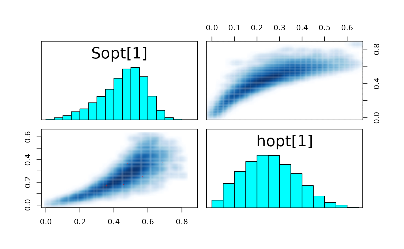
#> Warning in par(usr): argument 1 does not name a graphical parameter

#> Warning in par(usr): argument 1 does not name a graphical parameter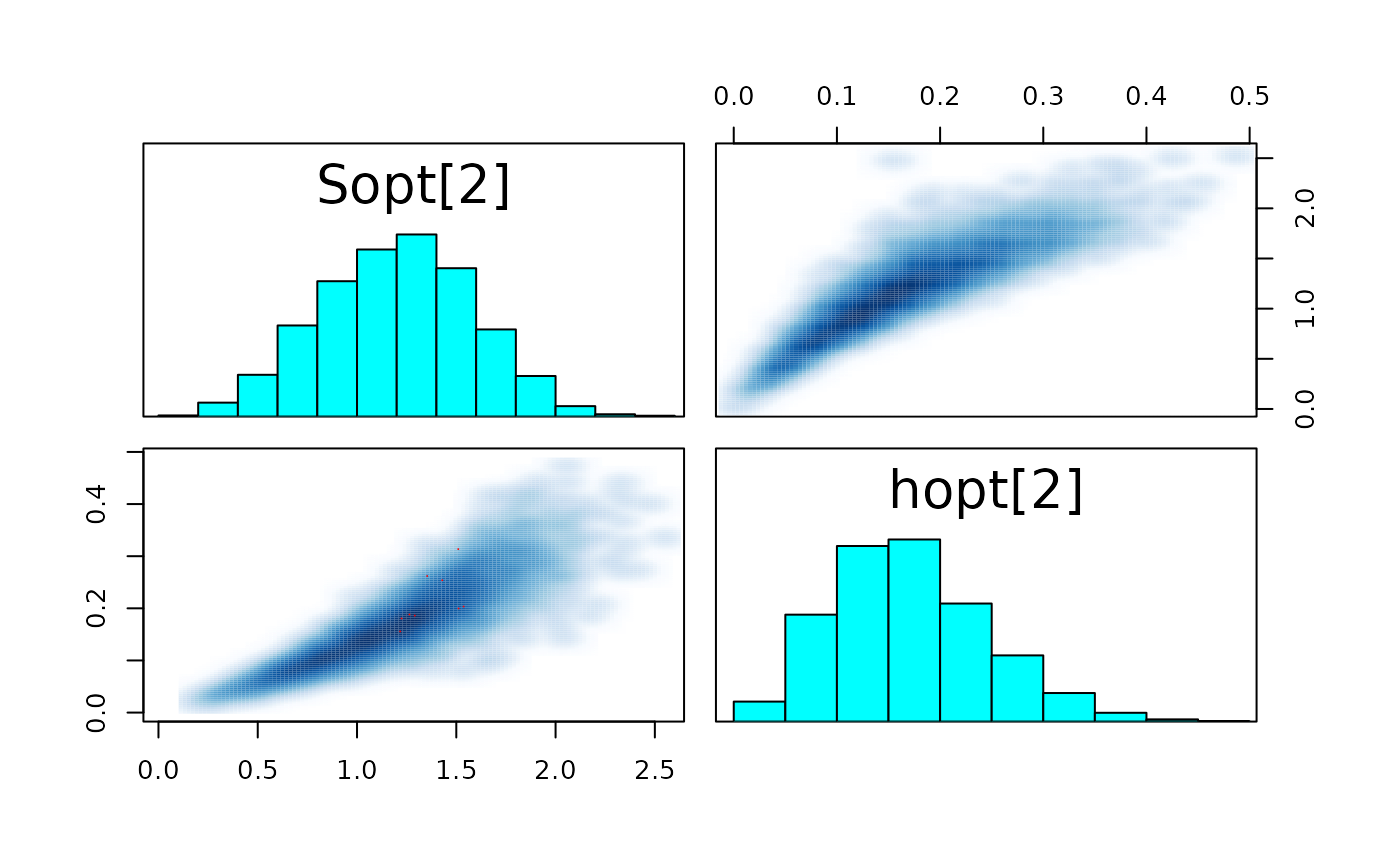
#> Warning in par(usr): argument 1 does not name a graphical parameter

#> Warning in par(usr): argument 1 does not name a graphical parameter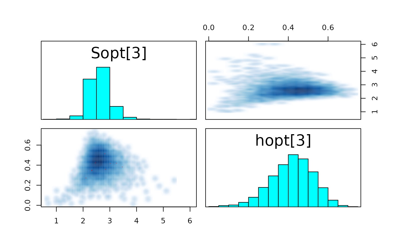
#> Warning in par(usr): argument 1 does not name a graphical parameter

#> Warning in par(usr): argument 1 does not name a graphical parameter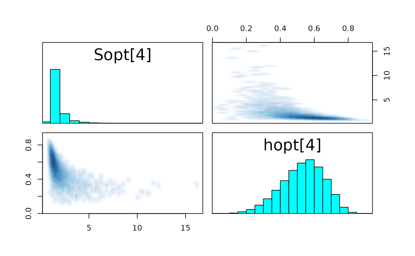
#> Warning in par(usr): argument 1 does not name a graphical parameter

#> Warning in par(usr): argument 1 does not name a graphical parameter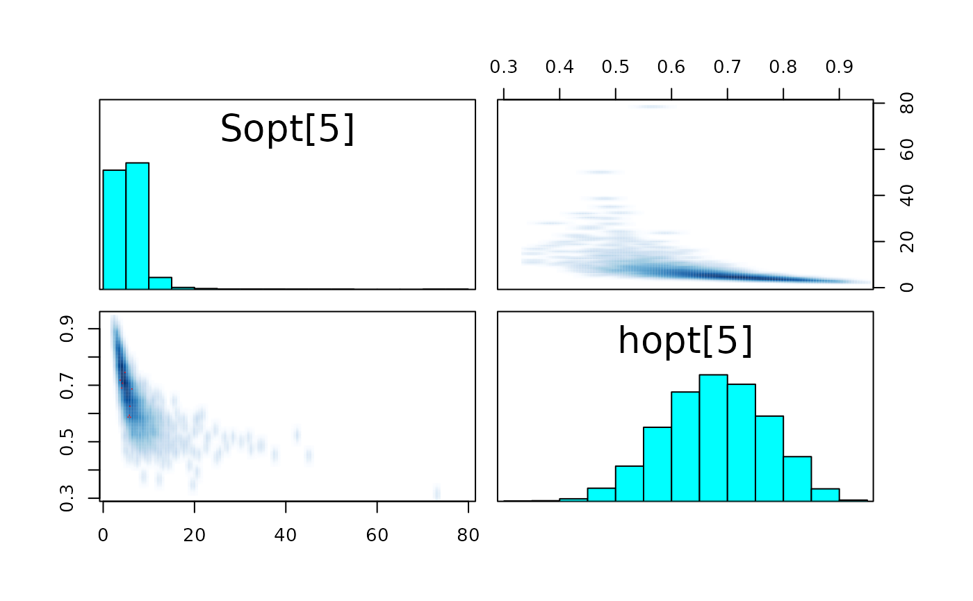
#> Warning in par(usr): argument 1 does not name a graphical parameter

#> Warning in par(usr): argument 1 does not name a graphical parameter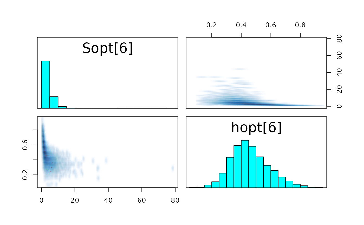
#> Warning in par(usr): argument 1 does not name a graphical parameter
#> Warning in KernSmooth::bkde2D(x, bandwidth = bandwidth, gridsize = nbin, :
#> Binning grid too coarse for current (small) bandwidth: consider increasing
#> 'gridsize'
#> Warning in par(usr): argument 1 does not name a graphical parameter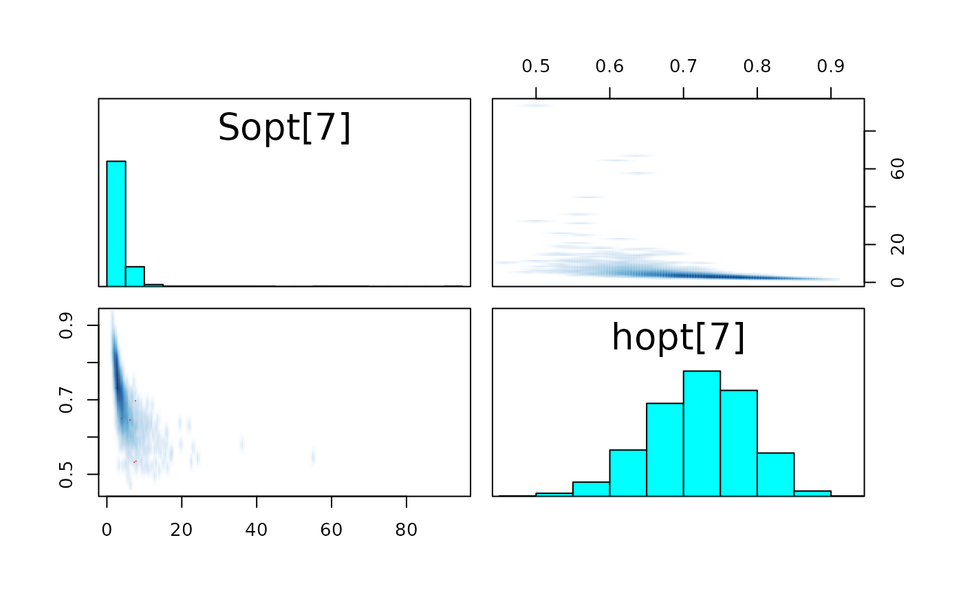
#> Warning in par(usr): argument 1 does not name a graphical parameter

#> Warning in par(usr): argument 1 does not name a graphical parameter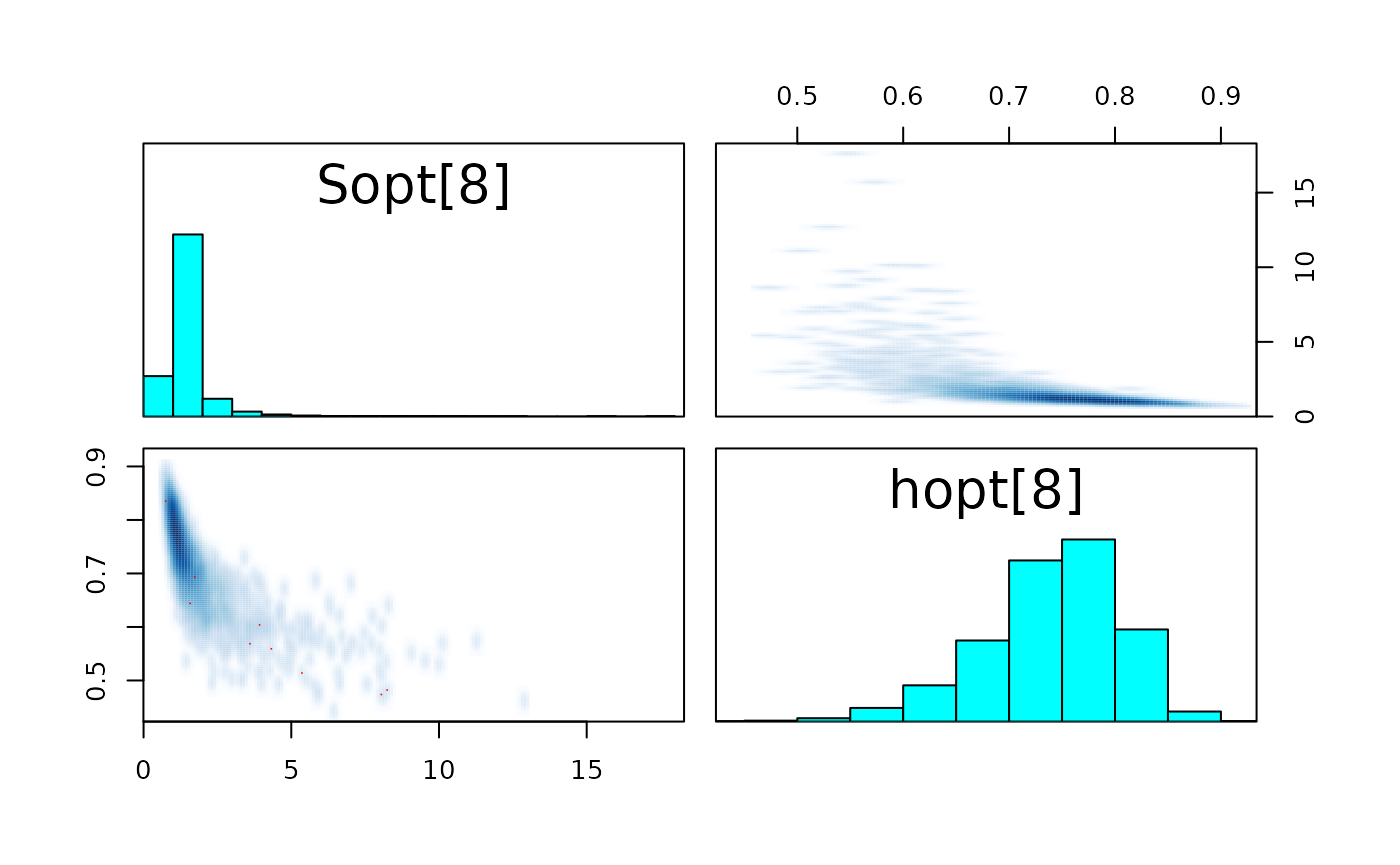
#> Warning in par(usr): argument 1 does not name a graphical parameter

#> Warning in par(usr): argument 1 does not name a graphical parameter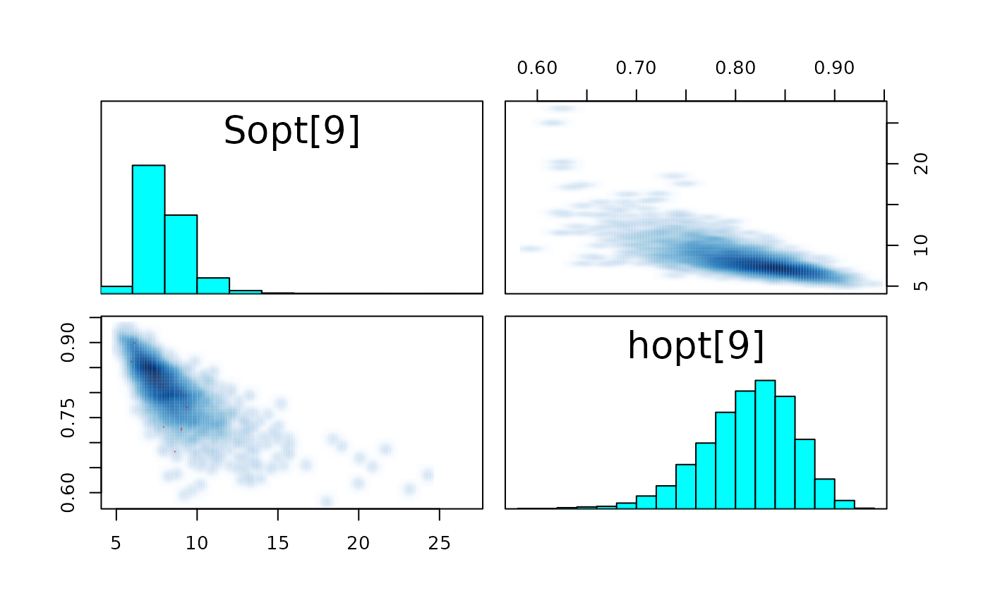
#> Warning in par(usr): argument 1 does not name a graphical parameter

#> Warning in par(usr): argument 1 does not name a graphical parameter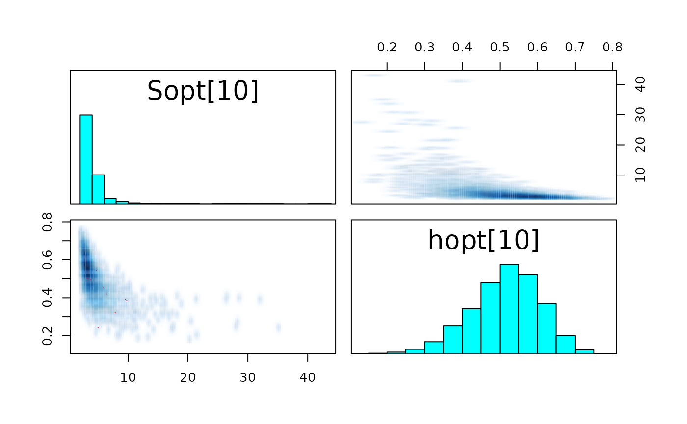
#> Warning in par(usr): argument 1 does not name a graphical parameter

#> Warning in par(usr): argument 1 does not name a graphical parameter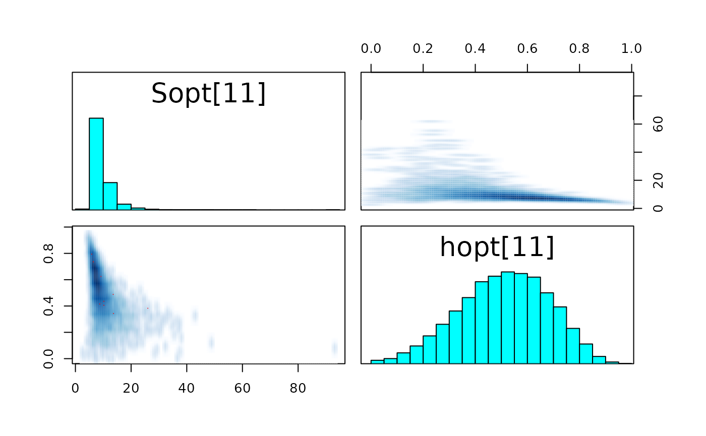
#> Warning in par(usr): argument 1 does not name a graphical parameter

#> Warning in par(usr): argument 1 does not name a graphical parameter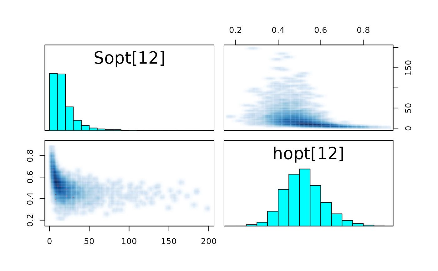
#> Warning in par(usr): argument 1 does not name a graphical parameter

#> Warning in par(usr): argument 1 does not name a graphical parameter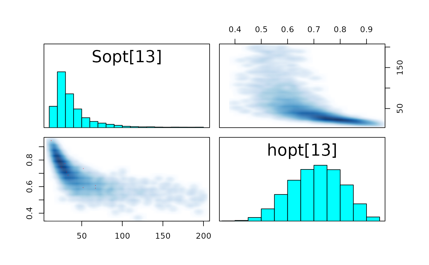
Results and analysis
names_ind <- SRSalmon$name_riv#c("Nivelle","Oir","Frome","Dee","Burrishoole","Lune","Bush",
#"Mourne","Faughan","Girnock Burn","North Esk","Laerdalselva","Ellidaar")

names_pred <- c("Nivelle","new 45?","Oir","new 50?","Frome","Dee","Burrishoole","Lune","new 55?","Bush",
"Mourne","Faughan","Girnock Burn","North Esk","new 60?","Laerdalselva","Ellidaar","new 65?")
dfw_hier <- extract_wider(fit_hier)
dfl_hier <- extract_longer(fit_hier) %>% mutate(Model = "Hierarchical")
Plotting Figure 9., Page 210
Sopt_hier <- dfl_hier %>%
  filter(str_detect(parameter, "Sopt\\.")) %>%
  mutate(Site = as_factor(str_sub(parameter, str_length("Sopt.")+1))) %>%
  group_by(Site) %>% summarise(Sopt_med = median(value))%>%
  select(Sopt_med) %>% as_vector()
hopt_hier <- fit_hier %>% extract_longer() %>%
  filter(str_detect(parameter, "hopt\\.")) %>%
  mutate(Site = as_factor(str_sub(parameter, str_length("hopt.")+1))) %>%
  group_by(Site) %>% summarise(hopt_med = median(value))%>%
  select(hopt_med) %>% as_vector()
Sopt_ind <- dfl_gamma %>%
  filter(str_detect(parameter, "Sopt\\.")) %>%
  mutate(Site = as_factor(str_sub(parameter, str_length("Sopt.")+1))) %>%
  group_by(Site) %>% summarise(Sopt_med = median(value))%>%
  select(Sopt_med) %>% as_vector()
hopt_ind <- dfl_gamma %>%
  filter(str_detect(parameter, "hopt\\.")) %>%
  mutate(Site = as_factor(str_sub(parameter, str_length("hopt.")+1))) %>%
  group_by(Site) %>% summarise(Sopt_med = median(value))%>%
  select(Sopt_med) %>% as_vector()
max_S <- sapply(seq_along(Sopt_ind), function(k) max(SRSalmon$S[SRSalmon$riv == k]))
Splot <- seq(0,100,length.out=1000)
Rplot_ind <- lapply(seq_along(Sopt_ind),
  function(k) {
    tibble(S = Splot[1:ceiling(15*max_S[k])],
           river = as_factor(names_ind[k]),
           R = exp( log(Splot[1:ceiling(15*max_S[k])]) + hopt_ind[k] -
                     log(1-hopt_ind[k]) - (hopt_ind[k]/Sopt_ind[k])*Splot[1:ceiling(15*max_S[k])] ))
    })%>%
  bind_rows()
Rplot_hier <- lapply(seq_along(Sopt_hier),
  function(k) {
    tibble(S = Splot[1:ceiling(15*max_S[k])],
           river = as_factor(names_ind[k]),
           R = exp( log(Splot[1:ceiling(15*max_S[k])]) + hopt_hier[k] -
                     log(1-hopt_hier[k]) - (hopt_hier[k]/Sopt_hier[k])*Splot[1:ceiling(15*max_S[k])] ))
    })%>%
  bind_rows()
tibble(R = SRSalmon$R, S = SRSalmon$S,
       river = factor(names_ind[SRSalmon$riv], levels = names_ind)) %>%
  ggplot() +
  aes(x = S, y = R) +
  geom_point() +
  facet_wrap(~ river, scales = "free") +
  geom_line(data = Rplot_hier, size = 1) +
  geom_line(data = Rplot_ind, size = 1, linetype = "dashed") +
  plot_theme +
  theme(axis.text.x =  element_text(angle = 0))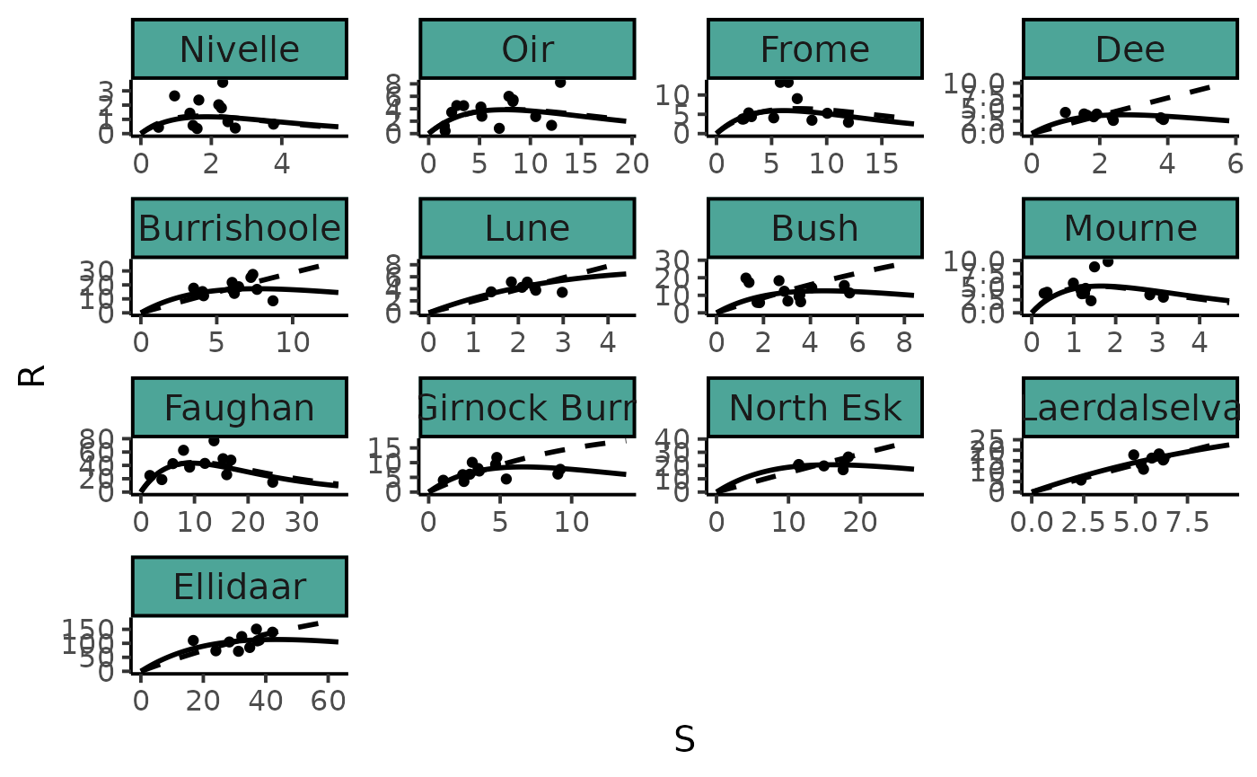
dfl <- bind_rows(dfl_gamma %>%  mutate(Model = "Independent"), dfl_hier)

dfl %>%
  filter(str_detect(parameter, "Sopt\\.")) %>%
  rename("S*" = value) %>%
  mutate(Site = as_factor(str_sub(parameter, str_length("Sopt.") + 1))) %>%
  ggplot() +
  aes(x = Site, y = log(`S*`), fill = Model ) +
  geom_boxplot(outlier.shape = NA, outlier.size = .25) +
  scale_x_discrete(labels = names_ind, guide = guide_axis(angle = 90)) +
  ylim(c(-3,6)) +
  scale_fill_manual(values = c("gray50", "gray90")) +
  ylab("log(S*)") +
  plot_theme
#> Warning: Removed 47 rows containing non-finite values (stat_boxplot).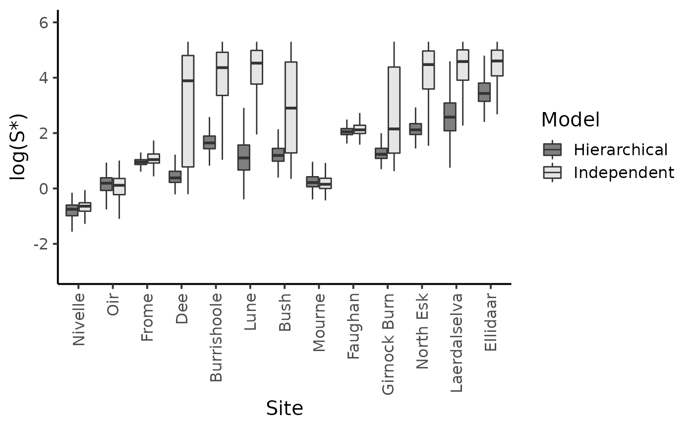
dfl %>%
  filter(str_detect(parameter, "hopt\\.")) %>%
  rename("h*" = value) %>%
  mutate(Site = as_factor(str_sub(parameter, str_length("hopt.") + 1))) %>%
  ggplot() +
  aes(x = Site, fill = Model, y = `h*`) +
  geom_boxplot(outlier.shape = NA,outlier.size = .25) +
  scale_x_discrete(labels = names_ind, guide = guide_axis(angle = 90)) +
  scale_fill_manual(values = c("gray50", "gray90"))+
  plot_theme
Plotting marginal posterior probability shapes of the parameters \(\alpha\), \(\beta\), \(\delta\), \(\kappa\), \(\sigma\), \(\tau_{h*}\) (Fig. 9.12 page 216)
dfl_hier %>%
  filter(parameter  %in% c("alpha", "beta", "delta", "kappa", "sigma", "sigma_h")) %>%
  mutate(parameter = replace(parameter, parameter == "sigma_h", "sigma[h]")) %>%
  ggplot() + aes(x = value) +
  geom_density(adjust = 2) +
  xlab("")+ ylab("")+
  facet_wrap(~ parameter, ncol = 2, scales = "free", labeller = label_parsed) +
  plot_theme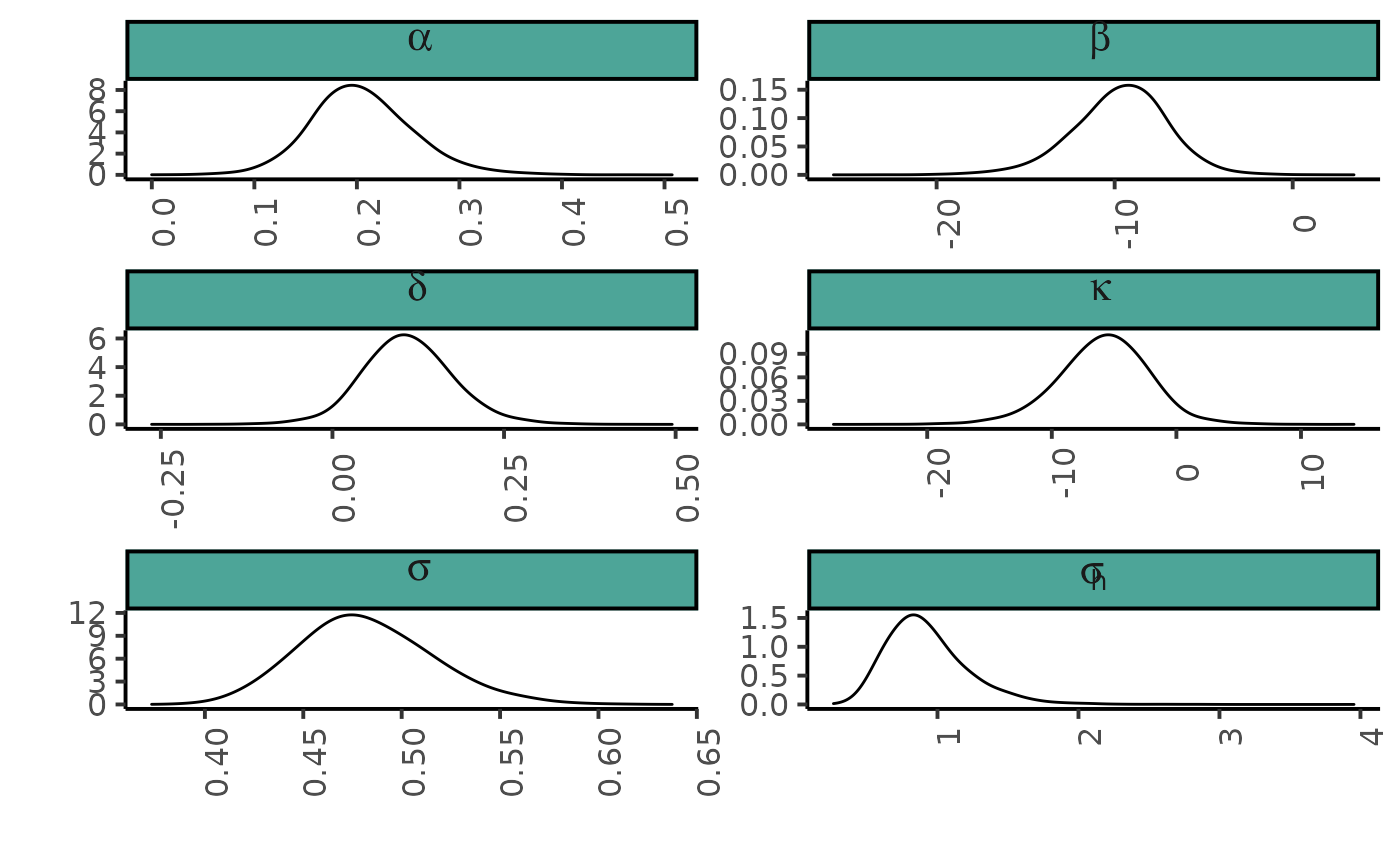
Marginal posterior distributions and posterior predictive of \(\log(S*)\) for the hierarchical model (fig. 9.13 page 217)
reg_param <- dfw_hier %>% select(alpha, beta) %>%
  summarise(med_a = median(alpha), med_b = median(beta))

fit_data <- dfl_hier %>%
  filter(str_detect(parameter, "Sopt\\.")) %>%
  rename("S*" = value) %>%
  mutate(id = as.factor(str_sub(parameter, str_length("Sopt.") + 1)),
    Latitude = SRSalmon$lat[as.numeric(str_sub(parameter, str_length("Sopt.") + 1))],
         type = "data")

fit_pred <- dfl_hier %>%
  filter(str_detect(parameter, "Sopt_")) %>%
  rename("S*" = value) %>%
  mutate(id = as.factor(str_sub(parameter, str_length("Sopt_")+1)),
    Latitude = SRSalmon$lat_pred[as.numeric(str_sub(parameter,str_length("Sopt_pred.") + 1))],
         type = "pred")

fit_data %>% bind_rows(fit_pred) %>%
  ggplot() +
  aes(x = Latitude, group = id,  y = log(`S*`), fill = type) +
  geom_boxplot(outlier.shape = NA,outlier.size = .25, varwidth = FALSE) +
#  scale_x_discrete(labels = names_ind, guide = guide_axis(angle = 90)) +
  scale_fill_manual(values = c("gray90", "gray50")) +
  geom_abline(slope = reg_param$med_a, intercept = reg_param$med_b) + #-reg_param$med_a*mean(data_hier$lat)) +
  ylim(c(-2,5)) +
  ylab("log(S*)") +
  plot_theme
#> Warning: Removed 1184 rows containing non-finite values (stat_boxplot).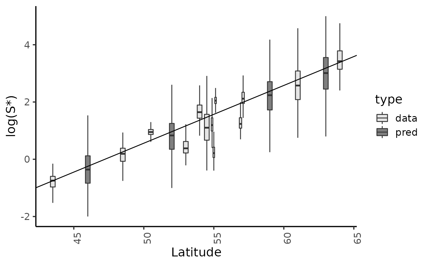
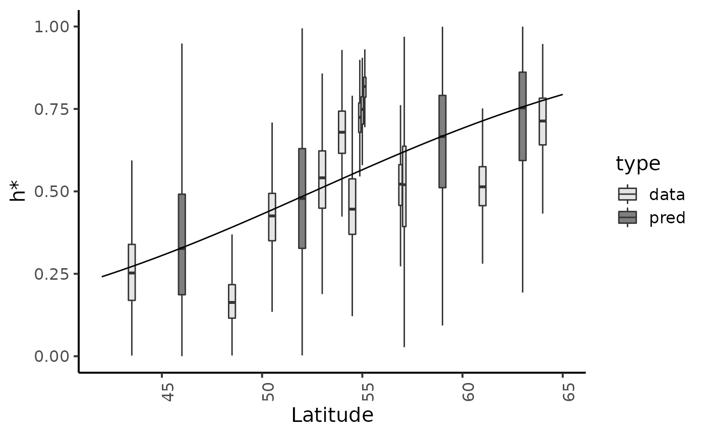
Marginal posterior distributions and posterior predictive of \(h*\) for the hierarchical model (fig. 9.14 page 218)
reg_param <- dfw_hier %>%
  select(delta, kappa) %>%
  summarise(med_d = median(delta), med_k = median(kappa))

fit_data <- dfl_hier %>%
  filter(str_detect(parameter, "^hopt\\.")) %>% # detect hopt. without logit_hopt.
  rename("h*" = value) %>%
  mutate(id = as.factor(str_sub(parameter, str_length("hopt.") + 1)),
    Latitude = SRSalmon$lat[as.numeric(str_sub(parameter, str_length("hopt.") + 1))],
         type = "data")

fit_pred <- dfl_hier %>%
  filter(str_detect(parameter, "^hopt_")) %>%
  rename("h*" = value) %>%
  mutate(id = as.factor(str_sub(parameter, str_length("hopt_") + 1)),
    Latitude = SRSalmon$lat_pred[as.numeric(str_sub(parameter, str_length("hopt_pred.") + 1))],
         type = "pred")

fit_data %>% bind_rows(fit_pred) %>%
  ggplot() +
  aes(x = Latitude, group = id,  y = `h*`, fill = type) +
  geom_boxplot(outlier.shape = NA,outlier.size = .25, varwidth = FALSE) +
#  scale_x_discrete(labels = names_ind, guide = guide_axis(angle = 90)) +
  scale_fill_manual(values = c("gray90", "gray50")) +
  annotate(x = seq(42, 65, .1),
           y = 1/(1+exp(-reg_param$med_d*seq(42, 65, .1) -reg_param$med_k)),
           geom = "line") +
  ylim(c(0,1)) +
  plot_theme