Biomass Production Model: The Namibian Hake Fishery

library(hbm4ecology)
#> Please visit the site https://Chabert-Liddell.github.io/hbm4ecology/articles/
#>                           for R case study.
library(rstan)
#> Loading required package: StanHeaders
#> Loading required package: ggplot2
#> rstan (Version 2.21.5, GitRev: 2e1f913d3ca3)
#> For execution on a local, multicore CPU with excess RAM we recommend calling
#> options(mc.cores = parallel::detectCores()).
#> To avoid recompilation of unchanged Stan programs, we recommend calling
#> rstan_options(auto_write = TRUE)
library(tidyverse)
#> ── Attaching packages ─────────────────────────────────────── tidyverse 1.3.1 ──
#> ✔ tibble  3.1.7     ✔ dplyr   1.0.9
#> ✔ tidyr   1.2.0     ✔ stringr 1.4.0
#> ✔ readr   2.1.2     ✔ forcats 0.5.1
#> ✔ purrr   0.3.4
#> ── Conflicts ────────────────────────────────────────── tidyverse_conflicts() ──
#> ✖ tidyr::extract() masks rstan::extract()
#> ✖ dplyr::filter()  masks stats::filter()
#> ✖ dplyr::lag()     masks stats::lag()
library(GGally)
#> Registered S3 method overwritten by 'GGally':
#>   method from   
#>   +.gg   ggplot2
library(posterior)
#> This is posterior version 1.2.1
#> 
#> Attaching package: 'posterior'
#> The following objects are masked from 'package:rstan':
#> 
#>     ess_bulk, ess_tail
#> The following objects are masked from 'package:stats':
#> 
#>     mad, sd, var
library(bayesplot)
#> This is bayesplot version 1.9.0
#> - Online documentation and vignettes at mc-stan.org/bayesplot
#> - bayesplot theme set to bayesplot::theme_default()
#>    * Does _not_ affect other ggplot2 plots
#>    * See ?bayesplot_theme_set for details on theme setting
#> 
#> Attaching package: 'bayesplot'
#> The following object is masked from 'package:posterior':
#> 
#>     rhat

The Namibian hake fishery

Let us consider as a first example the data from the Namibian hake fishery. Two hake species (Merlucius capensis and Merlucius paradoxus) are targeted by this fishery. The data analyzed here concern the fishery operating in zones 1.3 and 1.4 of the International Commission for the South-East Atlantic Fisheries (ICSEAF) from 1965 to 1988.

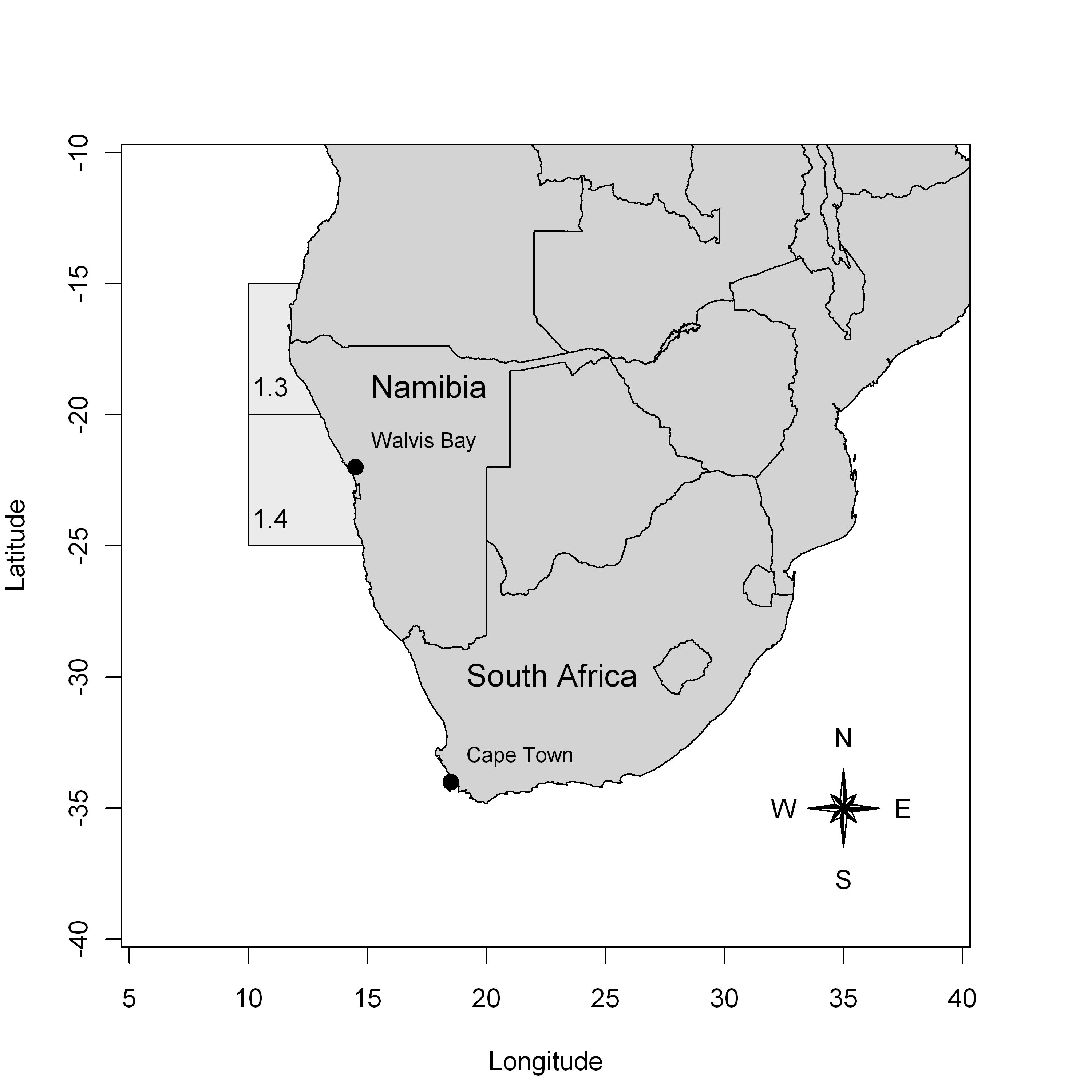
Figure 1 – Location of the ICSEAF fishery areas 1.3 and 1.4 in the Southeast coast of Africa.

For further details about the fishery, we refer to the report from the International Commission for Southeast Atlantic Fisheries (ICSEAF (1989)) or to Hilborn and Mangel (1997) and McAllister and Kirkwood (1998).

The two targeted species are pooled in the dataset. The catches concern the total annual commercial catches of hakes (in thousand tons) realized by large ocean-going trawlers operating in the ICSEAF zones 1.3 and 1.4. The catches per unit effort data (CPUEs) are the catches per hours of fishing for a specific class of Spanish trawlers. As the CPUEs are standardized, they are considered here as a reliable index of abundance for the Namibian hake stock.

We rely on these data to model the dynamics of hake stock biomass through dynamic Biomass Production Models (BPM). A dynamic BPM is a voluntarily crude but useful simplification of some harvested fish population dynamics (Hilborn and Walters (1992); Quinn and Deriso (1999)) that only aims at helping fisheries scientists to interpret the data (e.g., catches and abundance indices). Analyzing data through BPMs allows to assess how the fishery pressure has impacted the biomass. For instance, it provides answers to questions such as:

What is the maximum sustainable yield ($C_{MSY}$) and what are the past and current levels of yield sustainable with regards to the $C_{MSY}$?
How large was the abundance in year 1988 (the last year for the dataset) with reference to its level when the fishery began?
Could biomass level increase and yield be improved if more restrictive fishing quotas are imposed in the future?

The latter question is particularly important to test the performance of alternative management scenarios when efforts are being made to control the level of catches and promote sustainable harvest.

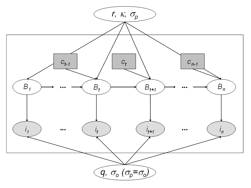
State-space modeling of a biomass production model

Process equation for the underlying dynamics of the biomass

$\frac{\mbox{d}B_t}{\mbox{d}t} = h(B_t)$
$h(B_t) = r\times B_t \times (1-\frac{B_t}{K})$ the production function
$r \sim Uniform(0.01, 3)$ is the population intrinsic growth
$K \sim Uniform(100, 15000)$ the carrying capacity

$h(B_t)$ is high when $B_t \approx 0$ and is null when $B_t = K$

Introducing the observed harvest between time $t$ and $t+1$, $c_t$ and a log normal random noise:

$B_{t+1} = (B_t + h(B_t) - c_t)\times e^{\epsilon_{t+1}}$
$\epsilon_{t+1} \sim Normal(0, \sigma^2_p)$, the environmental noise
$\sigma^2_p = \sigma^2$, with $\log(\sigma^2) \sim Uniform(-20,20)$
with $B_1 = K e^{\epsilon_1}$

Observation equation to link the data to the hidden process

$i_t = q \times B_t \times e^{\omega_t}$ the relative abundance index
$q$ such that $log(q) \sim Uniform (-20, 20)$ the catchability parameter
$\omega_t \sim Normal(0, \sigma_o^2)$ the observation noise
$\sigma^2_o = \sigma^2$, with $\log(\sigma^2) \sim Uniform(-20,20)$

In state-space modeling notation:

\[ \begin{cases} [Z_{t+1} | Z_t, \theta_1] \\ [y_t | Z_t, \theta_2] \end{cases} \] where

$Z_t = B_t$
$y_t = i_t$
$\theta_1 = \{r, K, \sigma_p \}$
$\theta_2 = \{q, \sigma_o \}$

Figure 2 – Directed acyclic graph of the state-space biomass production model

Sampling, results and analysis

Writing the model in Stan

stan_model_biomprod <- "
data {
  int N;
  int Year[N];
  vector<lower=0>[N] C;
  vector<lower=0>[N-1] I;
  int NF;
}

parameters {
  real<lower=0> r;
  real<lower=100, upper=15000> K;
  real<lower=-20, upper=20> log_q;
  real<lower=-20, upper=20> log_sig2;
  vector<lower=0>[N] P; //B_t/K
}

transformed parameters {
  real q;
  real sig;
  vector<lower=0>[N] B;
  
  q = exp(log_q);
  sig = sqrt(exp(log_sig2));
  B = K*P;
}

model {
  vector[N-1] h_P;

  P[1] ~ lognormal(0, sig);
  for (t in 1:(N-1)) {
      h_P[t] = r * K * P[t] * (1 - P[t]);
      P[t+1] ~ lognormal(log(P[t] + h_P[t]/K - C[t]/K), sig);
      I[t] ~ lognormal(log(q*K*P[t+1]), sig);
  }
}

generated quantities {
  // Abundance prediction
  vector[N] I_pred;
  vector[NF] B_pred100;
  vector[NF] B_pred500;
  
  for (t in 1:N) {
    I_pred[t] = lognormal_rng(log(q*K*P[t]), sig);
  }
  // Forecasting the biomass

  B_pred100[1] = (B[N] + r*B[N]*(1-B[N]/K) - 100) * lognormal_rng(0, sig);
  B_pred500[1] = (B[N] + r*B[N]*(1-B[N]/K) - 500)* lognormal_rng(0, sig);
  for (t in 1:(NF-1)) {
  B_pred100[t+1] = (B_pred100[t] + r*B_pred100[t]*(1-B_pred100[t]/K) - 100) * lognormal_rng(0, sig);
  B_pred500[t+1] = (B_pred500[t] + r*B_pred500[t]*(1-B_pred500[t]/K) - 500) * lognormal_rng(0, sig);
  }
} 

"

data(BioprodNamibianHake, package = "hbm4ecology")
dat_list <- BioprodNamibianHake
dat_list$I <- BioprodNamibianHake$I[2:25]
dat_list$NF <- 5

model_name <-"BiomProd_NamibianHake"
sm_hier <- stan_model(model_code =  stan_model_biomprod,
                 model_name =  model_name)
#> Trying to compile a simple C file
#> Running /usr/lib/R/bin/R CMD SHLIB foo.c
#> gcc -I"/usr/share/R/include" -DNDEBUG   -I"/home/chabertliddell/R/x86_64-pc-linux-gnu-library/4.2/Rcpp/include/"  -I"/home/chabertliddell/R/x86_64-pc-linux-gnu-library/4.2/RcppEigen/include/"  -I"/home/chabertliddell/R/x86_64-pc-linux-gnu-library/4.2/RcppEigen/include/unsupported"  -I"/home/chabertliddell/R/x86_64-pc-linux-gnu-library/4.2/BH/include" -I"/home/chabertliddell/R/x86_64-pc-linux-gnu-library/4.2/StanHeaders/include/src/"  -I"/home/chabertliddell/R/x86_64-pc-linux-gnu-library/4.2/StanHeaders/include/"  -I"/home/chabertliddell/R/x86_64-pc-linux-gnu-library/4.2/RcppParallel/include/"  -I"/home/chabertliddell/R/x86_64-pc-linux-gnu-library/4.2/rstan/include" -DEIGEN_NO_DEBUG  -DBOOST_DISABLE_ASSERTS  -DBOOST_PENDING_INTEGER_LOG2_HPP  -DSTAN_THREADS  -DBOOST_NO_AUTO_PTR  -include '/home/chabertliddell/R/x86_64-pc-linux-gnu-library/4.2/StanHeaders/include/stan/math/prim/mat/fun/Eigen.hpp'  -D_REENTRANT -DRCPP_PARALLEL_USE_TBB=1      -fpic  -g -O2 -fdebug-prefix-map=/build/r-base-zYgbYq/r-base-4.2.1=. -fstack-protector-strong -Wformat -Werror=format-security -Wdate-time -D_FORTIFY_SOURCE=2  -c foo.c -o foo.o
#> In file included from /home/chabertliddell/R/x86_64-pc-linux-gnu-library/4.2/RcppEigen/include/Eigen/Core:88,
#>                  from /home/chabertliddell/R/x86_64-pc-linux-gnu-library/4.2/RcppEigen/include/Eigen/Dense:1,
#>                  from /home/chabertliddell/R/x86_64-pc-linux-gnu-library/4.2/StanHeaders/include/stan/math/prim/mat/fun/Eigen.hpp:13,
#>                  from <command-line>:
#> /home/chabertliddell/R/x86_64-pc-linux-gnu-library/4.2/RcppEigen/include/Eigen/src/Core/util/Macros.h:628:1: error: unknown type name ‘namespace’
#>   628 | namespace Eigen {
#>       | ^~~~~~~~~
#> /home/chabertliddell/R/x86_64-pc-linux-gnu-library/4.2/RcppEigen/include/Eigen/src/Core/util/Macros.h:628:17: error: expected ‘=’, ‘,’, ‘;’, ‘asm’ or ‘__attribute__’ before ‘{’ token
#>   628 | namespace Eigen {
#>       |                 ^
#> In file included from /home/chabertliddell/R/x86_64-pc-linux-gnu-library/4.2/RcppEigen/include/Eigen/Dense:1,
#>                  from /home/chabertliddell/R/x86_64-pc-linux-gnu-library/4.2/StanHeaders/include/stan/math/prim/mat/fun/Eigen.hpp:13,
#>                  from <command-line>:
#> /home/chabertliddell/R/x86_64-pc-linux-gnu-library/4.2/RcppEigen/include/Eigen/Core:96:10: fatal error: complex: No such file or directory
#>    96 | #include <complex>
#>       |          ^~~~~~~~~
#> compilation terminated.
#> make: *** [/usr/lib/R/etc/Makeconf:168: foo.o] Error 1

fit_hier <- sampling(object = sm_hier,
                data = dat_list, 
                pars = NA, #params,
                chains = 4,
                init = lapply(seq(4), function(x)
                   list(P = rep(.5, 25))),
                iter = 4000, 
                warmup = 2000, 
                thin = 1,
                control = list("adapt_delta" = .9)
)
#> 
#> SAMPLING FOR MODEL 'BiomProd_NamibianHake' NOW (CHAIN 1).
#> Chain 1: 
#> Chain 1: Gradient evaluation took 2.4e-05 seconds
#> Chain 1: 1000 transitions using 10 leapfrog steps per transition would take 0.24 seconds.
#> Chain 1: Adjust your expectations accordingly!
#> Chain 1: 
#> Chain 1: 
#> Chain 1: Iteration:    1 / 4000 [  0%]  (Warmup)
#> Chain 1: Iteration:  400 / 4000 [ 10%]  (Warmup)
#> Chain 1: Iteration:  800 / 4000 [ 20%]  (Warmup)
#> Chain 1: Iteration: 1200 / 4000 [ 30%]  (Warmup)
#> Chain 1: Iteration: 1600 / 4000 [ 40%]  (Warmup)
#> Chain 1: Iteration: 2000 / 4000 [ 50%]  (Warmup)
#> Chain 1: Iteration: 2001 / 4000 [ 50%]  (Sampling)
#> Chain 1: Iteration: 2400 / 4000 [ 60%]  (Sampling)
#> Chain 1: Iteration: 2800 / 4000 [ 70%]  (Sampling)
#> Chain 1: Iteration: 3200 / 4000 [ 80%]  (Sampling)
#> Chain 1: Iteration: 3600 / 4000 [ 90%]  (Sampling)
#> Chain 1: Iteration: 4000 / 4000 [100%]  (Sampling)
#> Chain 1: 
#> Chain 1:  Elapsed Time: 2.58522 seconds (Warm-up)
#> Chain 1:                2.26416 seconds (Sampling)
#> Chain 1:                4.84939 seconds (Total)
#> Chain 1: 
#> 
#> SAMPLING FOR MODEL 'BiomProd_NamibianHake' NOW (CHAIN 2).
#> Chain 2: 
#> Chain 2: Gradient evaluation took 1.4e-05 seconds
#> Chain 2: 1000 transitions using 10 leapfrog steps per transition would take 0.14 seconds.
#> Chain 2: Adjust your expectations accordingly!
#> Chain 2: 
#> Chain 2: 
#> Chain 2: Iteration:    1 / 4000 [  0%]  (Warmup)
#> Chain 2: Iteration:  400 / 4000 [ 10%]  (Warmup)
#> Chain 2: Iteration:  800 / 4000 [ 20%]  (Warmup)
#> Chain 2: Iteration: 1200 / 4000 [ 30%]  (Warmup)
#> Chain 2: Iteration: 1600 / 4000 [ 40%]  (Warmup)
#> Chain 2: Iteration: 2000 / 4000 [ 50%]  (Warmup)
#> Chain 2: Iteration: 2001 / 4000 [ 50%]  (Sampling)
#> Chain 2: Iteration: 2400 / 4000 [ 60%]  (Sampling)
#> Chain 2: Iteration: 2800 / 4000 [ 70%]  (Sampling)
#> Chain 2: Iteration: 3200 / 4000 [ 80%]  (Sampling)
#> Chain 2: Iteration: 3600 / 4000 [ 90%]  (Sampling)
#> Chain 2: Iteration: 4000 / 4000 [100%]  (Sampling)
#> Chain 2: 
#> Chain 2:  Elapsed Time: 2.6589 seconds (Warm-up)
#> Chain 2:                3.28409 seconds (Sampling)
#> Chain 2:                5.94299 seconds (Total)
#> Chain 2: 
#> 
#> SAMPLING FOR MODEL 'BiomProd_NamibianHake' NOW (CHAIN 3).
#> Chain 3: 
#> Chain 3: Gradient evaluation took 1.4e-05 seconds
#> Chain 3: 1000 transitions using 10 leapfrog steps per transition would take 0.14 seconds.
#> Chain 3: Adjust your expectations accordingly!
#> Chain 3: 
#> Chain 3: 
#> Chain 3: Iteration:    1 / 4000 [  0%]  (Warmup)
#> Chain 3: Iteration:  400 / 4000 [ 10%]  (Warmup)
#> Chain 3: Iteration:  800 / 4000 [ 20%]  (Warmup)
#> Chain 3: Iteration: 1200 / 4000 [ 30%]  (Warmup)
#> Chain 3: Iteration: 1600 / 4000 [ 40%]  (Warmup)
#> Chain 3: Iteration: 2000 / 4000 [ 50%]  (Warmup)
#> Chain 3: Iteration: 2001 / 4000 [ 50%]  (Sampling)
#> Chain 3: Iteration: 2400 / 4000 [ 60%]  (Sampling)
#> Chain 3: Iteration: 2800 / 4000 [ 70%]  (Sampling)
#> Chain 3: Iteration: 3200 / 4000 [ 80%]  (Sampling)
#> Chain 3: Iteration: 3600 / 4000 [ 90%]  (Sampling)
#> Chain 3: Iteration: 4000 / 4000 [100%]  (Sampling)
#> Chain 3: 
#> Chain 3:  Elapsed Time: 2.91949 seconds (Warm-up)
#> Chain 3:                2.5367 seconds (Sampling)
#> Chain 3:                5.45619 seconds (Total)
#> Chain 3: 
#> 
#> SAMPLING FOR MODEL 'BiomProd_NamibianHake' NOW (CHAIN 4).
#> Chain 4: 
#> Chain 4: Gradient evaluation took 1.4e-05 seconds
#> Chain 4: 1000 transitions using 10 leapfrog steps per transition would take 0.14 seconds.
#> Chain 4: Adjust your expectations accordingly!
#> Chain 4: 
#> Chain 4: 
#> Chain 4: Iteration:    1 / 4000 [  0%]  (Warmup)
#> Chain 4: Iteration:  400 / 4000 [ 10%]  (Warmup)
#> Chain 4: Iteration:  800 / 4000 [ 20%]  (Warmup)
#> Chain 4: Iteration: 1200 / 4000 [ 30%]  (Warmup)
#> Chain 4: Iteration: 1600 / 4000 [ 40%]  (Warmup)
#> Chain 4: Iteration: 2000 / 4000 [ 50%]  (Warmup)
#> Chain 4: Iteration: 2001 / 4000 [ 50%]  (Sampling)
#> Chain 4: Iteration: 2400 / 4000 [ 60%]  (Sampling)
#> Chain 4: Iteration: 2800 / 4000 [ 70%]  (Sampling)
#> Chain 4: Iteration: 3200 / 4000 [ 80%]  (Sampling)
#> Chain 4: Iteration: 3600 / 4000 [ 90%]  (Sampling)
#> Chain 4: Iteration: 4000 / 4000 [100%]  (Sampling)
#> Chain 4: 
#> Chain 4:  Elapsed Time: 2.32494 seconds (Warm-up)
#> Chain 4:                2.429 seconds (Sampling)
#> Chain 4:                4.75394 seconds (Total)
#> Chain 4:

pars = c("r", "K", "q", "sig")
pairs(fit_hier, pars = c("r", "K", "q", "sig") )
#> Warning in par(usr): argument 1 does not name a graphical parameter

#> Warning in par(usr): argument 1 does not name a graphical parameter

#> Warning in par(usr): argument 1 does not name a graphical parameter

#> Warning in par(usr): argument 1 does not name a graphical parameter

traceplot(fit_hier, pars)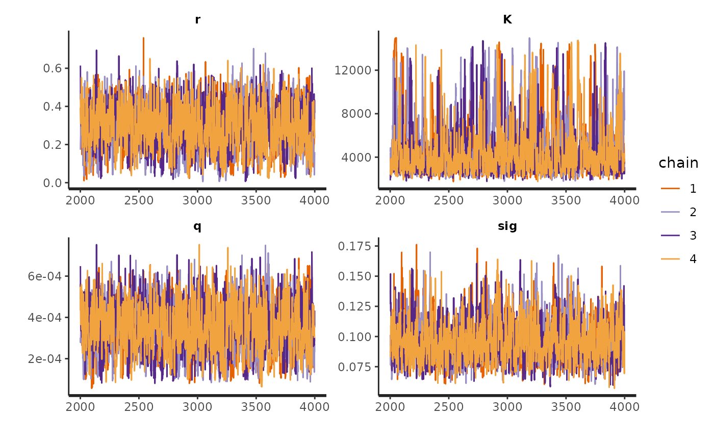

stan_rhat(fit_hier)
#> `stat_bin()` using `bins = 30`. Pick better value with `binwidth`.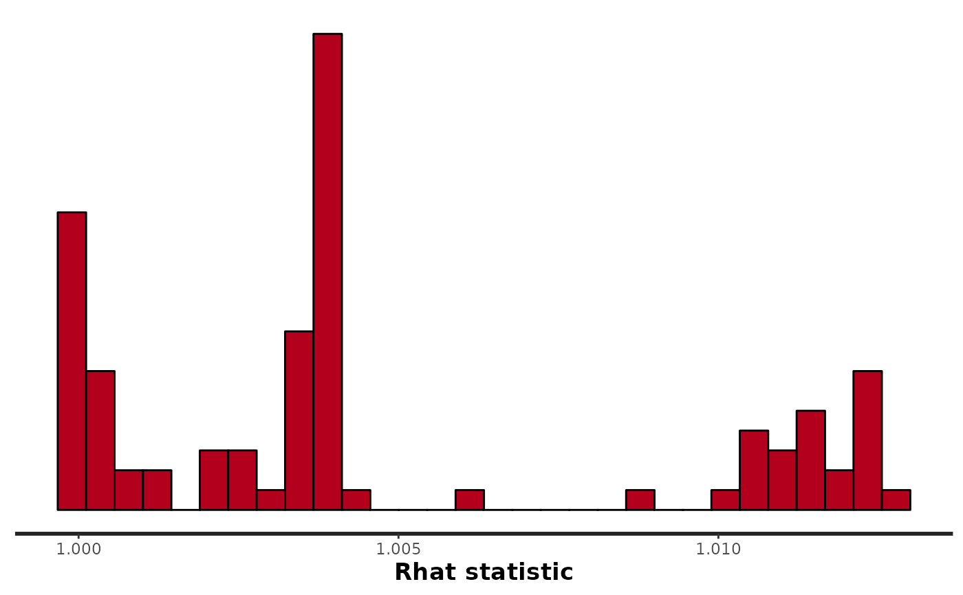

#mcmc_trace(fit_hier, pars = pars)
rhat(fit_hier, pars = pars)
#>        r        K        q      sig 
#> 1.003736 1.004431 1.003602 1.001359

pairs(fit_hier, pars = pars)
#> Warning in par(usr): argument 1 does not name a graphical parameter

#> Warning in par(usr): argument 1 does not name a graphical parameter

#> Warning in par(usr): argument 1 does not name a graphical parameter

#> Warning in par(usr): argument 1 does not name a graphical parameter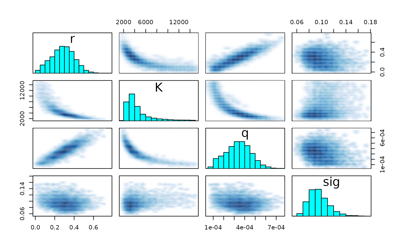

Analysis

df_w <- extract_wider(fit_hier)
df_l <- extract_longer(fit_hier)

df_w %>% 
  mutate(sig2 = sig * sig,
         B_MSY = K/2,
         C_MSY = r*K/4) %>% 
  select(r, K, q, sig2, B_MSY, C_MSY) %>% 
  pivot_longer(cols = everything(), names_to = "parameter") %>% 
  group_by(parameter) %>% 
#  filter(parameter %in% c("r", "K", "q", "sig")) %>% 
  summarise(Mean = mean(value),
            Sd = sd(value),
            `q.025` = quantile(value, .025),
            Median = median(value),
            `q.975` = quantile(value, .975)) %>% 
  knitr::kable(digits = 5)

parameter	Mean	Sd	q.025	Median	q.975
B_MSY	2289.02482	1214.22054	1136.20020	1880.48317	6101.15625
C_MSY	266.53760	54.75535	143.32551	268.44564	369.43237
K	4578.04964	2428.44108	2272.40039	3760.96635	12202.31249
q	0.00034	0.00012	0.00011	0.00034	0.00057
r	0.28277	0.11602	0.05890	0.28528	0.50560
sig2	0.00940	0.00334	0.00491	0.00874	0.01771

$B_{MSY} = \arg \max_{B} h(B) = K/2$
$C_{MSY} = g(B_{MSY}) = rK/4$

df_w %>% 
  mutate(C_MSY = r*K/4) %>% 
  ggpairs(c("r" , "K", "q", "C_MSY"))

df_l %>% 
  filter(str_detect(parameter, "I_pred")) %>% 
  mutate(
    id = as.numeric(str_sub(parameter, str_length("I_pred.")+1)),
    Year = BioprodNamibianHake$Year[id])  %>% 
  ggplot(aes(x = Year, y = value, group = Year)) +
  geom_boxplot(outlier.shape = NA) +
  annotate("line", x = BioprodNamibianHake$Year, y = BioprodNamibianHake$I) +
#  geom_line(data = dat, mapping = aes(y = I)) +
  ylim(c(0,2)) +
  ylab("Abundance indices") +
  scale_x_continuous(breaks = BioprodNamibianHake$Year,
                     labels = BioprodNamibianHake$Year, 
                     guide = guide_axis(angle = 90)) +
  theme_classic(base_size = 15)
#> Warning: Removed 197 rows containing non-finite values (stat_boxplot).
#> Warning: Removed 1 row(s) containing missing values (geom_path).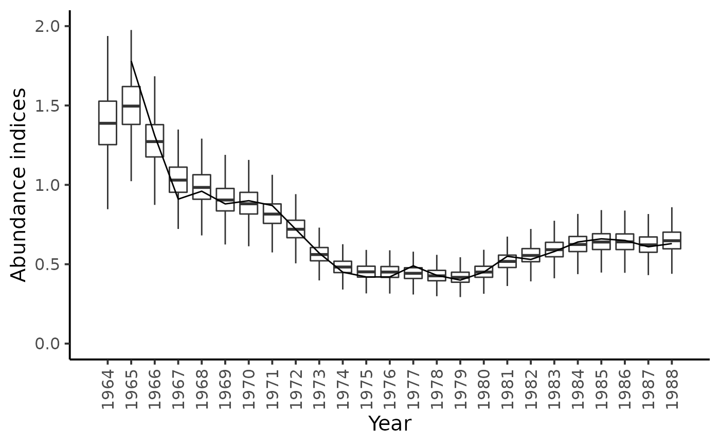

Forecasting the biomass for years 1989 to 1993

df_100 <- df_l %>% 
  filter(str_detect(parameter, "B_pred100\\.")) %>% 
  mutate(
    id = as.numeric(str_sub(parameter, str_length("B_pred100.")+1)),
    Year = seq(1989, 1993)[id], 
    data_type = "Pred100")    

df_500 <- df_l %>% 
  filter(str_detect(parameter, "B_pred500\\.")) %>% 
  mutate(
    id = as.numeric(str_sub(parameter, str_length("B_pred500.")+1)),
    Year = seq(1989, 1993)[id], 
    data_type = "Pred500")    

df_l %>%
  filter(str_detect(parameter, "B\\.")) %>%
  mutate(
    id = as.numeric(str_sub(parameter, str_length("B.")+1)),
    Year = BioprodNamibianHake$Year[id],
    data_type = "data")  %>%
  bind_rows(df_100, df_500) %>% 
  ggplot(aes(x = as_factor(Year), y = value)) +
  geom_boxplot(aes(fill = as_factor(data_type)),outlier.shape = NA, show.legend = FALSE) +
  ylim(c(0,10000)) +
  ylab("Biomass (x 1000 tons)") +
  xlab("Years") +
  scale_x_discrete( guide = guide_axis(angle = 90)) +
  scale_fill_manual(values = c("white", "gray90", "gray50"))+
  theme_classic(base_size = 15)
#> Warning: Removed 3541 rows containing non-finite values (stat_boxplot).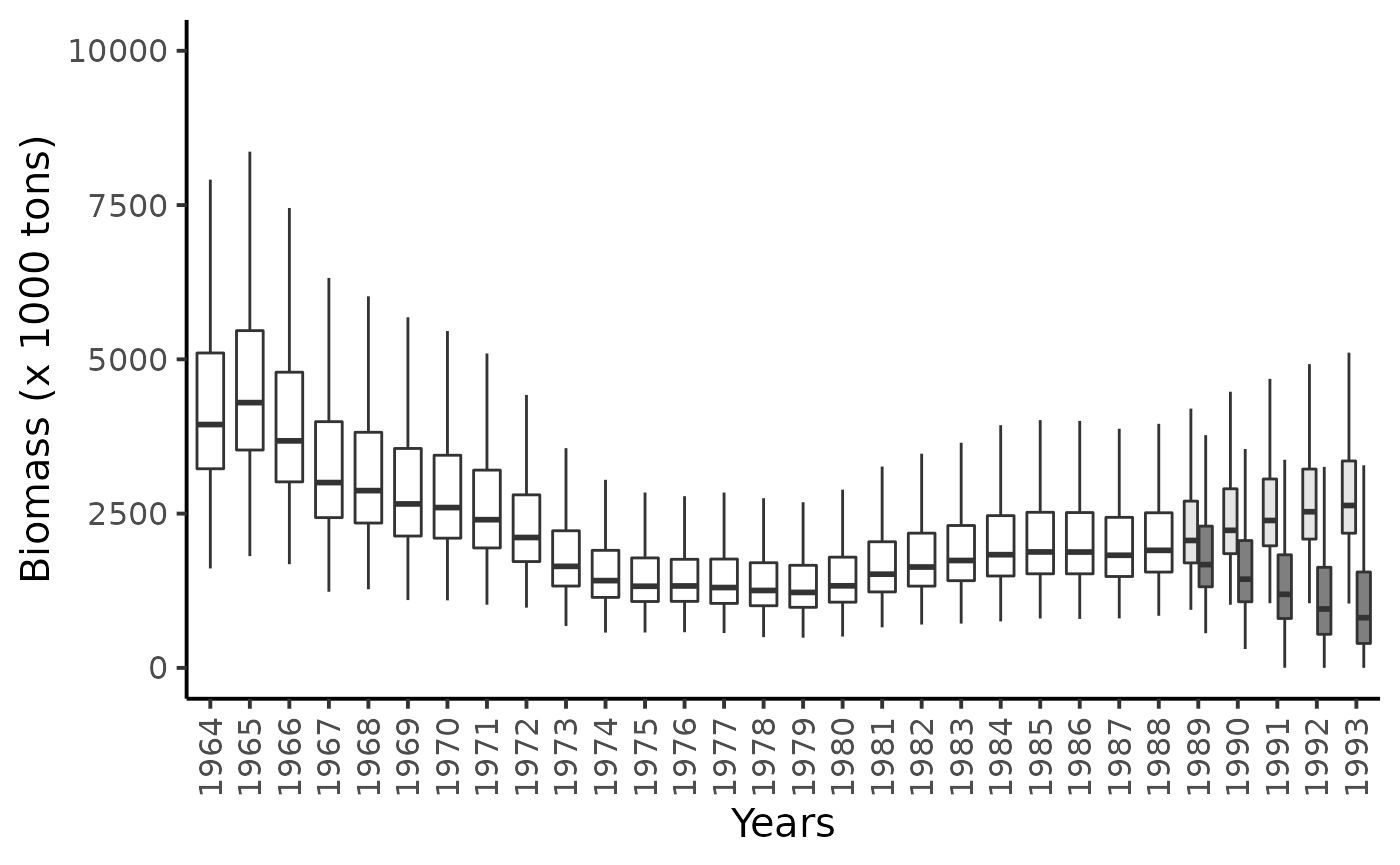

Comparing Schaefer-type versus Fox-type prodcution function

Recall that Schaefer type production function is given by: \[ h(B_t) = r \times B_t \times (1-\frac{B_t}{K}) \], with its associated fisheries management points: \[\begin{cases} C_{MSY} = \frac{r \times K}{4} \\ B_{MSY} = \frac{K}{2} \end{cases}\] The production function of the Fox model is the following: \[ $h(B_t) = r \times B_t \times (1-\frac{\log(B_t)}{\log(K)}) \], with its associated fisheries management points: \[\begin{cases} C_{MSY} = \frac{r \times K \times e^{-1}}{\log(K)} \\ B_{MSY} = K \times e^{-1} \end{cases}\]

stan_model_fox <- "
data {
  int N;
  int Year[N];
  vector<lower=0>[N] C;
  vector<lower=0>[N-1] I;
  int NF;
}

parameters {
  real<lower=0> r;
  real<lower=100, upper=15000> K;
  real<lower=-20, upper=20> log_q;
  real<lower=-20, upper=20> log_sig2;

  vector<lower=0>[N] P; //B_t/K
}

transformed parameters {
  real q;
  real sig;
  vector<lower=0>[N] B;
  
  q = exp(log_q);
  sig = sqrt(exp(log_sig2));
  B = K*P;
}

model {
  vector[N-1] h_P;

  P[1] ~ lognormal(0, sig);
  for (t in 1:(N-1)) {
      h_P[t] = r * K * P[t] * (1 - log(K*P[t])/log(K));
      P[t+1] ~ lognormal(log(P[t] + h_P[t]/K - C[t]/K), sig);
      I[t] ~ lognormal(log_q+log(K*P[t+1]), sig);
  }
}

generated quantities {
  // Abundance prediction
  vector[N] I_pred;
  vector[NF] B_pred100;
  vector[NF] B_pred500;
  
  for (t in 1:N) {
    I_pred[t] = lognormal_rng(log(q*B[t]), sig);
  }
  // Forecasting the biomass

  B_pred100[1] = (B[N] + r*B[N]*(1-log(B[N])/log(K)) - 100) * exp(normal_rng(0, sig));
  B_pred500[1] = (B[N] + r*B[N]*(1-log(B[N])/log(K)) - 500)* exp(normal_rng(0, sig));
  for (t in 1:(NF-1)) {
  B_pred100[t+1] = (B_pred100[t] + r*B_pred100[t]*(1-log(B_pred100[t])/log(K)) - 100) * exp(normal_rng(0, sig));
  B_pred500[t+1] = (B_pred500[t] + r*B_pred500[t]*(1-log(B_pred500[t])/log(K)) - 500) * exp(normal_rng(0, sig));
  }
} 

"

model_name <-"BiomProd_NamibianHake_fox"
sm_fox <- stan_model(model_code =  stan_model_fox,
                 model_name =  model_name)
#> Trying to compile a simple C file
#> Running /usr/lib/R/bin/R CMD SHLIB foo.c
#> gcc -I"/usr/share/R/include" -DNDEBUG   -I"/home/chabertliddell/R/x86_64-pc-linux-gnu-library/4.2/Rcpp/include/"  -I"/home/chabertliddell/R/x86_64-pc-linux-gnu-library/4.2/RcppEigen/include/"  -I"/home/chabertliddell/R/x86_64-pc-linux-gnu-library/4.2/RcppEigen/include/unsupported"  -I"/home/chabertliddell/R/x86_64-pc-linux-gnu-library/4.2/BH/include" -I"/home/chabertliddell/R/x86_64-pc-linux-gnu-library/4.2/StanHeaders/include/src/"  -I"/home/chabertliddell/R/x86_64-pc-linux-gnu-library/4.2/StanHeaders/include/"  -I"/home/chabertliddell/R/x86_64-pc-linux-gnu-library/4.2/RcppParallel/include/"  -I"/home/chabertliddell/R/x86_64-pc-linux-gnu-library/4.2/rstan/include" -DEIGEN_NO_DEBUG  -DBOOST_DISABLE_ASSERTS  -DBOOST_PENDING_INTEGER_LOG2_HPP  -DSTAN_THREADS  -DBOOST_NO_AUTO_PTR  -include '/home/chabertliddell/R/x86_64-pc-linux-gnu-library/4.2/StanHeaders/include/stan/math/prim/mat/fun/Eigen.hpp'  -D_REENTRANT -DRCPP_PARALLEL_USE_TBB=1      -fpic  -g -O2 -fdebug-prefix-map=/build/r-base-zYgbYq/r-base-4.2.1=. -fstack-protector-strong -Wformat -Werror=format-security -Wdate-time -D_FORTIFY_SOURCE=2  -c foo.c -o foo.o
#> In file included from /home/chabertliddell/R/x86_64-pc-linux-gnu-library/4.2/RcppEigen/include/Eigen/Core:88,
#>                  from /home/chabertliddell/R/x86_64-pc-linux-gnu-library/4.2/RcppEigen/include/Eigen/Dense:1,
#>                  from /home/chabertliddell/R/x86_64-pc-linux-gnu-library/4.2/StanHeaders/include/stan/math/prim/mat/fun/Eigen.hpp:13,
#>                  from <command-line>:
#> /home/chabertliddell/R/x86_64-pc-linux-gnu-library/4.2/RcppEigen/include/Eigen/src/Core/util/Macros.h:628:1: error: unknown type name ‘namespace’
#>   628 | namespace Eigen {
#>       | ^~~~~~~~~
#> /home/chabertliddell/R/x86_64-pc-linux-gnu-library/4.2/RcppEigen/include/Eigen/src/Core/util/Macros.h:628:17: error: expected ‘=’, ‘,’, ‘;’, ‘asm’ or ‘__attribute__’ before ‘{’ token
#>   628 | namespace Eigen {
#>       |                 ^
#> In file included from /home/chabertliddell/R/x86_64-pc-linux-gnu-library/4.2/RcppEigen/include/Eigen/Dense:1,
#>                  from /home/chabertliddell/R/x86_64-pc-linux-gnu-library/4.2/StanHeaders/include/stan/math/prim/mat/fun/Eigen.hpp:13,
#>                  from <command-line>:
#> /home/chabertliddell/R/x86_64-pc-linux-gnu-library/4.2/RcppEigen/include/Eigen/Core:96:10: fatal error: complex: No such file or directory
#>    96 | #include <complex>
#>       |          ^~~~~~~~~
#> compilation terminated.
#> make: *** [/usr/lib/R/etc/Makeconf:168: foo.o] Error 1

fit_fox <- sampling(object = sm_fox,
                data = dat_list, 
                pars = NA, #params,
                chains = 4,
                 init = lapply(seq(4), function(x)
                   list(K = 5000, r = 0.3, P = rep(.5, 25))),
                iter = 5000, 
                warmup = 2500, 
                thin = 1#,
              #  control = list("max_treedepth" = 12)
)
#> 
#> SAMPLING FOR MODEL 'BiomProd_NamibianHake_fox' NOW (CHAIN 1).
#> Chain 1: 
#> Chain 1: Gradient evaluation took 2.8e-05 seconds
#> Chain 1: 1000 transitions using 10 leapfrog steps per transition would take 0.28 seconds.
#> Chain 1: Adjust your expectations accordingly!
#> Chain 1: 
#> Chain 1: 
#> Chain 1: Iteration:    1 / 5000 [  0%]  (Warmup)
#> Chain 1: Iteration:  500 / 5000 [ 10%]  (Warmup)
#> Chain 1: Iteration: 1000 / 5000 [ 20%]  (Warmup)
#> Chain 1: Iteration: 1500 / 5000 [ 30%]  (Warmup)
#> Chain 1: Iteration: 2000 / 5000 [ 40%]  (Warmup)
#> Chain 1: Iteration: 2500 / 5000 [ 50%]  (Warmup)
#> Chain 1: Iteration: 2501 / 5000 [ 50%]  (Sampling)
#> Chain 1: Iteration: 3000 / 5000 [ 60%]  (Sampling)
#> Chain 1: Iteration: 3500 / 5000 [ 70%]  (Sampling)
#> Chain 1: Iteration: 4000 / 5000 [ 80%]  (Sampling)
#> Chain 1: Iteration: 4500 / 5000 [ 90%]  (Sampling)
#> Chain 1: Iteration: 5000 / 5000 [100%]  (Sampling)
#> Chain 1: 
#> Chain 1:  Elapsed Time: 3.20107 seconds (Warm-up)
#> Chain 1:                3.73471 seconds (Sampling)
#> Chain 1:                6.93578 seconds (Total)
#> Chain 1: 
#> 
#> SAMPLING FOR MODEL 'BiomProd_NamibianHake_fox' NOW (CHAIN 2).
#> Chain 2: 
#> Chain 2: Gradient evaluation took 1.8e-05 seconds
#> Chain 2: 1000 transitions using 10 leapfrog steps per transition would take 0.18 seconds.
#> Chain 2: Adjust your expectations accordingly!
#> Chain 2: 
#> Chain 2: 
#> Chain 2: Iteration:    1 / 5000 [  0%]  (Warmup)
#> Chain 2: Iteration:  500 / 5000 [ 10%]  (Warmup)
#> Chain 2: Iteration: 1000 / 5000 [ 20%]  (Warmup)
#> Chain 2: Iteration: 1500 / 5000 [ 30%]  (Warmup)
#> Chain 2: Iteration: 2000 / 5000 [ 40%]  (Warmup)
#> Chain 2: Iteration: 2500 / 5000 [ 50%]  (Warmup)
#> Chain 2: Iteration: 2501 / 5000 [ 50%]  (Sampling)
#> Chain 2: Iteration: 3000 / 5000 [ 60%]  (Sampling)
#> Chain 2: Iteration: 3500 / 5000 [ 70%]  (Sampling)
#> Chain 2: Iteration: 4000 / 5000 [ 80%]  (Sampling)
#> Chain 2: Iteration: 4500 / 5000 [ 90%]  (Sampling)
#> Chain 2: Iteration: 5000 / 5000 [100%]  (Sampling)
#> Chain 2: 
#> Chain 2:  Elapsed Time: 3.2095 seconds (Warm-up)
#> Chain 2:                3.54702 seconds (Sampling)
#> Chain 2:                6.75653 seconds (Total)
#> Chain 2: 
#> 
#> SAMPLING FOR MODEL 'BiomProd_NamibianHake_fox' NOW (CHAIN 3).
#> Chain 3: 
#> Chain 3: Gradient evaluation took 1.7e-05 seconds
#> Chain 3: 1000 transitions using 10 leapfrog steps per transition would take 0.17 seconds.
#> Chain 3: Adjust your expectations accordingly!
#> Chain 3: 
#> Chain 3: 
#> Chain 3: Iteration:    1 / 5000 [  0%]  (Warmup)
#> Chain 3: Iteration:  500 / 5000 [ 10%]  (Warmup)
#> Chain 3: Iteration: 1000 / 5000 [ 20%]  (Warmup)
#> Chain 3: Iteration: 1500 / 5000 [ 30%]  (Warmup)
#> Chain 3: Iteration: 2000 / 5000 [ 40%]  (Warmup)
#> Chain 3: Iteration: 2500 / 5000 [ 50%]  (Warmup)
#> Chain 3: Iteration: 2501 / 5000 [ 50%]  (Sampling)
#> Chain 3: Iteration: 3000 / 5000 [ 60%]  (Sampling)
#> Chain 3: Iteration: 3500 / 5000 [ 70%]  (Sampling)
#> Chain 3: Iteration: 4000 / 5000 [ 80%]  (Sampling)
#> Chain 3: Iteration: 4500 / 5000 [ 90%]  (Sampling)
#> Chain 3: Iteration: 5000 / 5000 [100%]  (Sampling)
#> Chain 3: 
#> Chain 3:  Elapsed Time: 4.82213 seconds (Warm-up)
#> Chain 3:                3.37023 seconds (Sampling)
#> Chain 3:                8.19236 seconds (Total)
#> Chain 3: 
#> 
#> SAMPLING FOR MODEL 'BiomProd_NamibianHake_fox' NOW (CHAIN 4).
#> Chain 4: 
#> Chain 4: Gradient evaluation took 1.8e-05 seconds
#> Chain 4: 1000 transitions using 10 leapfrog steps per transition would take 0.18 seconds.
#> Chain 4: Adjust your expectations accordingly!
#> Chain 4: 
#> Chain 4: 
#> Chain 4: Iteration:    1 / 5000 [  0%]  (Warmup)
#> Chain 4: Iteration:  500 / 5000 [ 10%]  (Warmup)
#> Chain 4: Iteration: 1000 / 5000 [ 20%]  (Warmup)
#> Chain 4: Iteration: 1500 / 5000 [ 30%]  (Warmup)
#> Chain 4: Iteration: 2000 / 5000 [ 40%]  (Warmup)
#> Chain 4: Iteration: 2500 / 5000 [ 50%]  (Warmup)
#> Chain 4: Iteration: 2501 / 5000 [ 50%]  (Sampling)
#> Chain 4: Iteration: 3000 / 5000 [ 60%]  (Sampling)
#> Chain 4: Iteration: 3500 / 5000 [ 70%]  (Sampling)
#> Chain 4: Iteration: 4000 / 5000 [ 80%]  (Sampling)
#> Chain 4: Iteration: 4500 / 5000 [ 90%]  (Sampling)
#> Chain 4: Iteration: 5000 / 5000 [100%]  (Sampling)
#> Chain 4: 
#> Chain 4:  Elapsed Time: 2.824 seconds (Warm-up)
#> Chain 4:                2.90512 seconds (Sampling)
#> Chain 4:                5.72912 seconds (Total)
#> Chain 4:
#> Warning in validityMethod(object): The following variables have undefined
#> values: B_pred100[3],The following variables have undefined values:
#> B_pred100[4],The following variables have undefined values: B_pred100[5],The
#> following variables have undefined values: B_pred500[3],The following
#> variables have undefined values: B_pred500[4],The following variables have
#> undefined values: B_pred500[5],The following variables have undefined values:
#> B_pred100[2],The following variables have undefined values: B_pred500[2]. Many
#> subsequent functions will not work correctly.
#> Warning: There were 28 divergent transitions after warmup. See
#> https://mc-stan.org/misc/warnings.html#divergent-transitions-after-warmup
#> to find out why this is a problem and how to eliminate them.
#> Warning: Examine the pairs() plot to diagnose sampling problems

pars = c("q", "K", "r", "sig")
stan_rhat(fit_fox)
#> `stat_bin()` using `bins = 30`. Pick better value with `binwidth`.
#> Warning: Removed 1 rows containing non-finite values (stat_bin).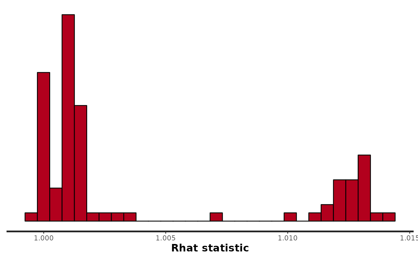

pairs(fit_fox, pars = pars)
#> Warning in par(usr): argument 1 does not name a graphical parameter
#> Warning in par(usr): argument 1 does not name a graphical parameter

#> Warning in par(usr): argument 1 does not name a graphical parameter

#> Warning in par(usr): argument 1 does not name a graphical parameter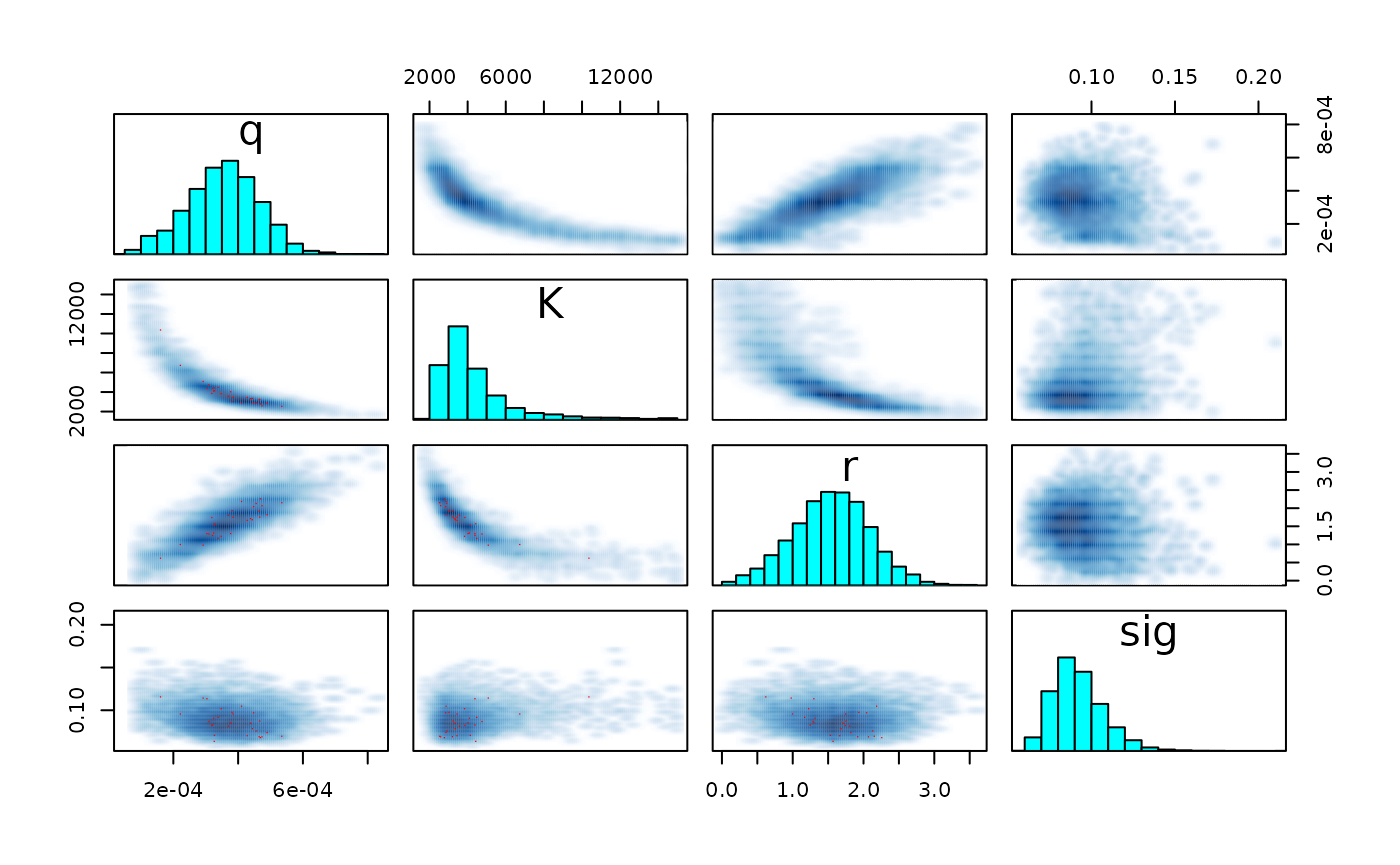

df_l_fox <- extract_longer(fit_fox) %>% 
  mutate(model = "Fox")

df_100_fox <- df_l_fox %>% 
  filter(str_detect(parameter, "B_pred100\\.")) %>% 
  mutate(
    id = as.numeric(str_sub(parameter, str_length("B_pred100.")+1)),
    Year = seq(1989, 1993)[id], 
    data_type = "Pred100")  

df_l %>% mutate(model = "Schaefer") %>% 
  bind_rows(df_l_fox) %>% 
    filter(str_detect(parameter, "B\\.")) %>%
  mutate(
    id = as.numeric(str_sub(parameter, str_length("B.")+1)),
    Year = BioprodNamibianHake$Year[id],
    data_type = "data")  %>%
  bind_rows(df_100 %>%  mutate(model = "Schaefer"), df_100_fox) %>% 
  ggplot(aes(x = as_factor(Year), y = value)) +
  geom_boxplot(aes(fill = model),outlier.shape = NA) +
  geom_vline(xintercept = 25.5, linetype = "dashed") +
  ylim(c(0,10000)) +
  ylab("Biomass (x 1000 tons)") + xlab("Years") +
  scale_x_discrete( guide = guide_axis(angle = 90)) +
  scale_fill_manual(values = c("gray90", "gray50"))+
  theme_classic(base_size = 15)
#> Warning: Removed 3214 rows containing non-finite values (stat_boxplot).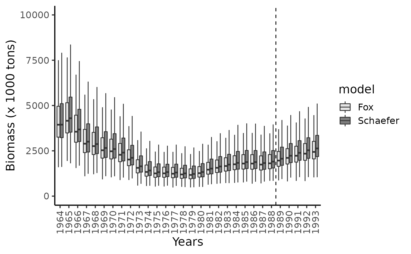

df_w %>% mutate(C_MSY = r*K/4,
                Model = "Schaefer") %>% 
  bind_rows(extract_wider(fit_fox) %>% 
              mutate(C_MSY = r*K*exp(-1)/log(K),
                     Model = "Fox")) %>% 
  ggplot(aes(x = C_MSY, linetype = Model)) +
  geom_density(adjust = 2) +
  theme_classic(base_size = 15)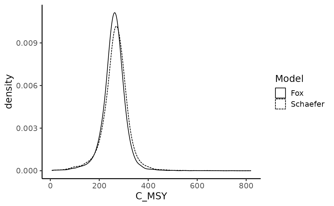

df_w %>% mutate(B_MSY = K/2,
                Model = "Schaefer") %>% 
  bind_rows(extract_wider(fit_fox) %>% 
              mutate(B_MSY = K*exp(-1),
                     Model = "Fox")) %>% 
  ggplot(aes(x = B_MSY, linetype = Model)) +
  geom_density(adjust = 2) +
  theme_classic(base_size = 15)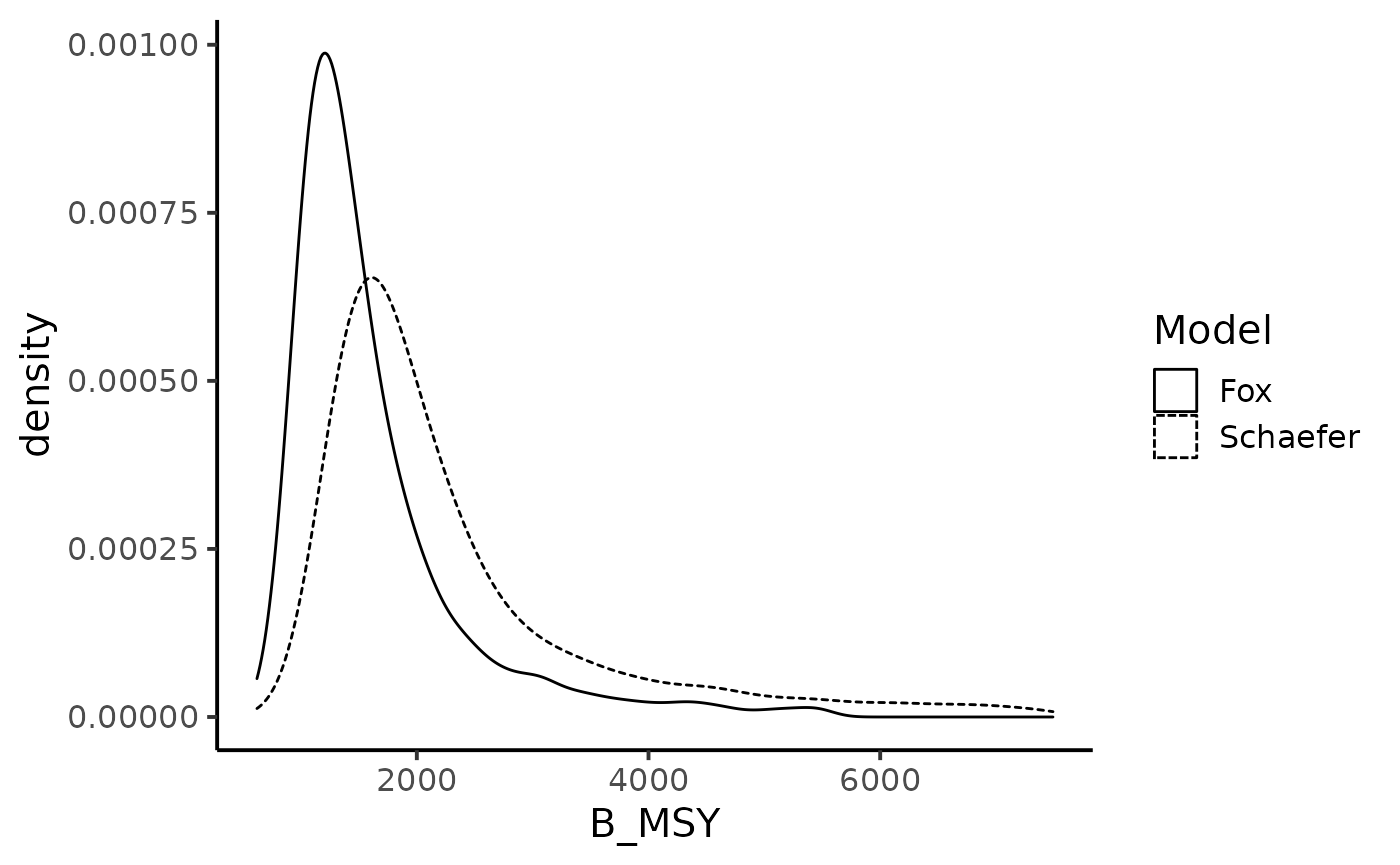

We now look at the chance of the biomass level to be under the Maximum Sustainable Yields biomass. Under the Schaefer production model:

df_w %>% mutate(B_MSY = K/2) %>% 
  mutate(Depletion_100 = B_pred100.5 < B_MSY,
         Depletion_500 = B_pred500.5 < B_MSY) %>% 
  summarise(`Depletion (100K scenario)` = mean(Depletion_100),
            `Depletion (500K scenario)` = mean(Depletion_500)) %>% 
  knitr::kable()

Depletion (100K scenario)	Depletion (500K scenario)
0.1185	0.967375

Under the Fox production model:

fit_fox %>% extract_wider() %>% 
  mutate(B_MSY = K*exp(-1)) %>% 
  mutate(Depletion_100 = B_pred100.5 < B_MSY,
         Depletion_500 = B_pred500.5 < B_MSY) %>% 
  summarise(`Depletion (100K scenario)` = mean(Depletion_100, na.rm = TRUE),
            `Depletion (500K scenario)` = mean(Depletion_500, na.rm = TRUE)) %>% 
  knitr::kable()

Depletion (100K scenario)	Depletion (500K scenario)
0.0197	0.9264136

References

Hilborn, R., and M. Mangel. 1997. The Ecological Detective Confronting Models with Data. Vol. 28. Monographs in Population Biology. Princeton, New Jersey: Princeton University Press.

Hilborn, R., and C. J. Walters. 1992. Quantitative Fisheries Stocks Assessment: Choice, Dynamics & Uncertainty. Col. Natural Resources. New York: Chapman & Hall.

ICSEAF. 1989. “Historical Series Data Selected for Cape Hake Assessment.” ICSEAF Documents. Vol. SAC/89/Doc./3 (10 pp). ICSEAF.

McAllister, M. K., and G. P. Kirkwood. 1998. “Bayesian Stock Assessment: A Review and Example Application Using the Logistic Model.” ICES Journal of Marine Science 55: 1031–60.

Quinn, J. J., I, and R. B. Deriso. 1999. “Quantitative Fish Dynamics.” In. Biological Resource Management. Oxford, New York: Oxford University Press.

Chapter 11.2